DeepSeek新框架DSpark原论文拆解
引言
这次我们要拆解的是 deepseek 联合北京大学发表的官方投机解码框架,但是对于论文原文大家阅读都比较困难,所以我下面就以「原文 English → 中文翻译 → 拆解解释」的格式来为大家深度解读一下整篇论文到底讲了什么,话不多说,我们下面就以原文开始
DSpark: Confidence-Scheduled Speculative Decoding with Semi-Autoregressive Generation
原文标题:DSpark: Confidence-Scheduled Speculative Decoding with Semi-Autoregressive Generation
作者:Xin Cheng, Xingkai Yu, Chenze Shao, Jiashi Li, Yunfan Xiong, Yi Qian, Jiaqi Zhu 等 (北京大学 + DeepSeek-AI)
来源:arXiv preprint, 2026-06-27
链接:https://www.alphaxiv.org/abs/2026.dspark
Abstract
原文:
Speculative decoding accelerates Large Language Model (LLM) inference by decoupling draft generation from target verification. While recent parallel drafters efficiently propose long token sequences in a single forward pass, they suffer from rapid acceptance decay due to a lack of inter-token dependencies. Furthermore, indiscriminately verifying these extended blocks wastes critical batch capacity on tokens with high rejection risks, severely degrading throughput in high-concurrency serving systems. We introduce DSpark, a speculative decoding framework that unifies high-throughput parallel generation with adaptive, load-aware verification. To maintain draft quality, DSpark utilizes a semi-autoregressive architecture—coupling a parallel backbone with a lightweight sequential module—to introduce intra-block dependency modeling and mitigate suffix decay. To optimize system efficiency, DSpark employs confidence-scheduled verification, dynamically tailoring the verification length for each request based on estimated prefix survival probabilities and engine-specific throughput profiles. On offline benchmarks across diverse domains, DSpark substantially improves the accepted length over state-of-the-art autoregressive and parallel drafters. When deployed within the DeepSeek-V4 serving system under live user traffic, DSpark successfully mitigates verification waste. Compared to the established production baseline (MTP-1), DSpark accelerates per-user generation speeds by 60%–85% at matched throughput levels. More importantly, by preventing severe throughput degradation under strict interactivity constraints, it enables performance tiers that were previously unattainable, shifting the Pareto frontier of our serving system. To facilitate community progress, we open-source the DSpark checkpoints alongside DeepSpec, an algorithm-driven training repository for speculative decoding.
中文翻译:
投机解码通过将草稿生成(draft generation)与目标验证(target verification)解耦,加速了大语言模型的推理。然而,近期的并行草稿生成器虽然在单次前向传播中高效生成长 token 序列,但因缺乏 token 间的相互依赖,遭受快速的接受率衰减(acceptance decay)。此外,不加区分地验证这些扩展块,会浪费关键批处理容量在高拒绝风险的 token 上,严重降低高并发服务系统的吞吐量。我们提出了 DSpark,一个将高吞吐并行生成与自适应、负载感知验证相统一的投机解码框架。为了维持草稿质量,DSpark 采用了半自回归架构——将并行主干与轻量级序列模块耦合——引入块内依赖建模以缓解后缀衰减(suffix decay)。为了优化系统效率,DSpark 使用了置信度调度验证,基于估计的前缀存活概率和引擎特定的吞吐量曲线,动态调整每个请求的验证长度。在跨多个领域的离线基准测试中,DSpark 在接受的 token 长度上大幅超越了最先进的自回归和并行草稿生成器。当部署在 DeepSeek-V4 服务系统中面对真实用户流量时,DSpark 成功缓解了验证浪费。与生产基线 MTP-1 相比,DSpark 在匹配吞吐量水平下将单用户生成速度提升了 60%–85%。更重要的是,通过在严格的交互性约束下防止严重的吞吐量退化,它实现了以前无法达到的性能等级,将我们服务系统的 Pareto 前沿向外推移。为促进社区为了推动进展,我们将 DSpark 检查点与 DeepSpec(一种由算法驱动的)一同开源投机解码的训练库。1. 引言大语言模型(LLMs)以自回归方式生成文本:每个新的词元都需要基于所有先前的词元进行一次完整的前向传播,这使得推理延迟与输出长度成正比。由此导致的低GPU利用率和高用户感知等待时间构成。
[!note] 整段一句话版
现在大模型推理太慢了,投机解码让"小模型先猜、大模型后验"来加速。但并行草稿器猜的词之间没有关联,越猜越不靠谱;而且不管三七二十一全验证,浪费服务器的并发能力。DSpark 用"半自回归"(semi-autoregressive)让猜测更准确,用"置信度调度"(confidence-scheduled verification)让验证更聪明,在 DeepSeek-V4 实测加速 60-85%。
[!tip] "投机解码"是什么?——考场打草稿类比
想象你在做大题:正式答案每写一步都要反复确认,很慢。但你可以先在草稿上飞速写 5 行,然后正式核对一次:
- 草稿第 1-3 行对了 ✅ → 直接抄到正式答案上,赚了 3 步
- 草稿第 4 行错了 ❌ → 这一行按正式答案改,后面的草稿全扔
关键保证:最终抄到正式答案纸上的,和"不用草稿纸直接写"完全一样。只是过程更快,质量不变。
这跟量化、蒸馏不同:量化(INT8)和蒸馏(训练小模型)会改变模型输出,有质量损失;投机解码不改模型,只改推理路径。
1. Introduction
原文:
Large Language Models (LLMs) generate text autoregressively: each new token requires a full forward pass conditioned on all preceding tokens, making inference latency proportional to the output length. The resulting low GPU utilization and high user-perceived waiting time constitute a primary bottleneck in production LLM serving, particularly for latency-sensitive scenarios such as real-time conversational assistants and multi-turn agentic workflows.
中文翻译:
大语言模型以自回归(autoregressive)方式生成文本:每个新 token 都需要在依赖所有前置 token 的条件下执行一次完整的前向传播,使得推理延迟与输出长度成正比。由此导致的 GPU 低利用率和用户高感知等待时间,构成了生产环境 LLM 服务的主要瓶颈,尤其对于延迟敏感的场景,如实时对话助手和多轮 Agent 工作流。
[!note] 什么叫"自回归"?
自回归 = 自己的输出当自己的输入。大模型每生成一个词,都要把前面所有已经生成的词重新读一遍,才能决定下一个词是什么。就像写作文:写完第一句,要带着第一句的意思想第二句;写完第二句,带着前两句的意思想第三句……字字出神,所以叫"逐 token 生成"。这有个大问题:生成 1000 个字就要跑 1000 次推理。GPU 大部分时间在等——就像一个厨师,每次只能炒一个菜,但灶台同时能炒 10 个菜,9 个灶口空着。
原文:
Speculative decoding (Chen et al., 2023; Leviathan et al., 2023) offers a principled solution: a lightweight draft model proposes a block of candidate tokens, and the full-size target model verifies the entire block in a single forward pass via rejection sampling, accepting the longest prefix consistent with the target distribution and appending one bonus token. Because verification is parallel and the acceptance rule preserves the target distribution exactly, speculative decoding accelerates generation without any quality loss.
中文翻译:
投机性解码(Chen等人,2023年;Leviathan等人,2023年)提供了一个有原则的解决方案:一个轻量级的草稿模型提出一组候选标记,全尺寸目标模型通过拒绝采样在单次前向传播中验证整个组,接受与目标分布一致的最长前缀并追加一个奖励标记。由于验证是并行的,且接受规则能精确保持目标分布,因此推测解码在不损失任何质量的情况下加速了生成过程。草案模型的设计决定了起草延迟和接受度之间的权衡速率。早期的草稿生成器是自回归的(Cheng等人,2024;Li等人,2024b),对每个在先前采样的标记上的位置。然而,它们的起草延迟随块大小线性增长,迫使这些方法使用短块和浅层架构。为了打破这种顺序瓶颈,并行起草者(Cai等人,2024;Chen等人,2026;Liu等人,2026a)已成为一种极具吸引力的替代方案:所有草稿位置在单次前向传播中生成,使得草稿延迟几乎与块大小无关。这种结构优势理论上允许并行草稿生成器高效地生成更长的草稿块。然而,充分释放大型并行草稿块的潜力会带来两个关键瓶颈——一个是生成质量方面,另一个是系统效率方面。首先,由于并行草稿生成器独立预测每个位置,它们无法对标记间的依赖关系进行建模
在一个块内。这种独立性导致多模态碰撞和快速接受衰减。
[!note] "无质量损失"是什么意思?
用投机解码生成的文本,和用原始逐字生成方式生成的文本,统计上完全一致。不是说每次输出一模一样,而是概率分布一样——就像"考试用草稿纸算"和"心算"的结果分布相同,只是草稿纸更快。
原文:
The design of the draft model governs the trade-off between drafting latency and acceptance rate. Early drafters are autoregressive, conditioning each position on previously sampled tokens. However, their drafting latency grows linearly with the block size, forcing these methods to use short blocks and shallow architectures. To break this sequential bottleneck, parallel drafters have emerged as a compelling alternative: all draft positions are produced in a single forward pass, making drafting latency nearly independent of block size. This structural advantage theoretically allows parallel drafters to efficiently generate substantially longer draft blocks.
中文翻译:
草稿模型的设计决定了草稿延迟(drafting latency)与接受率(acceptance rate)之间的权衡。早期的草稿生成器是自回归的,每个位置都依赖之前采样的 token。然而,它们的草稿延迟与块大小线性增长,迫使这些方法使用短块和浅层架构。为了打破这一顺序瓶颈,并行草稿生成器成为有吸引力的替代方案:所有草稿位置在一次前向传播中生成,使草稿延迟几乎与块大小无关。这种结构优势理论上允许并行绘图器高效地生成更长的草图块。
原文:
However, fully unlocking the potential of large parallel draft blocks introduces two critical bottlenecks—one in generation quality, and the other in system efficiency. First, because parallel drafters predict each position independently, they cannot model inter-token dependencies within a block. This independence leads to multi-modal collisions and rapid acceptance decay at later positions (Gu et al., 2018; Huang et al., 2022b). Second, determining the optimal verification length remains a challenge. While parallel generation easily produces long draft blocks, indiscriminately verifying all proposed tokens degrades system throughput, particularly under high-concurrency workloads (Hu et al., 2026; Liu et al., 2024c). The ideal verification length varies along two axes. On the data side, structured requests like code naturally sustain higher acceptance rates than open-ended chat (Abramovich et al., 2026; Xia et al., 2024). On the system side, verifying extra tokens is nearly free under light loads. Under heavy loads, however, verifying tokens with a high rejection risk occupies critical batch capacity that could otherwise serve other active requests (Liu et al., 2024b; Wu et al., 2025).
中文翻译:
然而,充分释放大型并行起草块的全部潜力会引入两个关键的瓶颈一-一个在于生成质量另一个在于系统效率。首先,由于并行起草者独立预测每个位置,它们无法模拟块内代币之间的相互依赖关系。这种独立性会导致多模态冲突,并在后续位置处导致接受率的迅速下降(Gu等,2018;Huang等,2022b)。其次,确定最优验证长度的过程仍具挑战性。尽管并行生成容易生成较长的起草块,但不加区分地验证所有提议的代币会降低系统的吞吐量,尤其是在高并发工作负载下(Hu等,2026;Liu等,2024c)。理想的验证长度会根据两个轴的不同而有所变化。从数据层面来看,结构化请求(如代码)自然比开放式聊天具有更高的接受率(Abramovich等,2026;Xia等,2024)。从系统层面来看,在负载较轻的情况下,验证额外令牌几乎是不需要成本的。然而,在负载较重的情况下,验证具有较高拒收风险的令牌会占用关键的批量处理能力,而这些处理能力原本可用于处理其他活跃请求(Liu等,2024b;Wu等,2025)。
[!warning] 具体来说——两个坑
坑① Suffix Decay(后缀衰减):并行草稿器猜词时,第 1 个词通常不错,但第 5、第 8 个词越来越差,因为词之间没有关联。题目是"今天天气",并行草稿可能猜出"今天天气很好所以我们"——到第 5 个词"我们"就很奇怪了,"很好"和"所以"之间没有逻辑关系。论文数据显示,并行草稿后几个位置接受率从 80% 降到 20%。坑② 验证浪费:不管忙闲、不管草稿质量,都固定验 N 个 token。忙的时候(比如 1000 个请求同时在跑),验一堆没用的 token 挤占了服务器处理其他请求的能力。
原文:
To address these bottlenecks, we introduce DSpark, a speculative decoding framework that unifies high-throughput parallel generation with adaptive, load-aware verification. At its core, DSpark is designed to resolve the inherent trade-offs in draft generation and verification through two complementary mechanisms:
• First, to overcome the lack of inter-token dependencies, DSpark adopts a semi-autoregressive architecture. It keeps the computationally expensive draft backbone fully parallel, appending only a lightweight serial output head to inject local transition information. This design preserves the drafting speed of parallel models while significantly mitigating suffix decay.
• Second, to resolve the system-level bottleneck, DSpark employs confidence-scheduled verification. By coupling a confidence head—which estimates per-position prefix survival probabilities—with a hardware-aware scheduler, DSpark dynamically tailors the verification length for each request. This scheduler leverages real-time engine throughput profiles to route target verification budget only toward tokens with the highest expected return.
中文翻译:
为了解决这些瓶颈,我们提出了 DSpark,一个将高吞吐并行生成与自适应、负载感知验证相统一的投机解码框架。DSpark 通过两个互补机制解决草稿生成与验证中的固有权衡:
• 首先,为了克服词元间依赖关系的缺失,DSpark采用了半自回归架构。它保持计算成本高昂的草稿主干完全并行,仅附加一个轻量级的串行输出头来注入局部转移信息。这种设计在保留并行模型草稿速度的同时,显著缓解了后缀衰减问题。
• 其次,为解决系统级瓶颈,DSpark采用置信度调度验证。通过将估计每个位置前缀存活概率的置信度头与硬件感知调度器相结合,DSpark为每个请求动态调整验证长度。该调度器利用实时引擎吞吐量概况,仅将目标验证预算分配给预期回报最高的令牌。
[!note] 用"快闪店+质检员"类比
- 并行主干(parallel backbone) = 快闪店:10 个员工同时备菜(每个位置同时处理)——快
- 序列输出头(sequential head) = 质检员:拿着前一个员工的菜看一眼,调整自己的出品——准
- 质检员只有 1 个(单层 decoder),所以只增加很少的时间,但让菜品前后连贯多了
- • 半自回归架构:保持计算昂贵的草稿主干完全并行,只附加一个轻量级串行输出头注入局部转移信息。
• 置信度调度验证:将估计每个位置前缀存活概率的置信度头与硬件感知调度器耦合,动态调整每个请求的验证长度。
原文:
We extensively evaluate DSpark across both controlled offline benchmarks and productionscale online deployments. On controlled offline benchmarks—spanning mathematical reasoning, code generation, and daily chat—DSpark consistently outperforms strong baselines. Specifically, across the Qwen3-4B, 8B, and 14B target models (Yang et al., 2025), it improves the macro-average accepted length over the autoregressive Eagle3 (Li et al., 2026b) by 30.9%, 26.7%, and 30.0%, and over the parallel DFlash (Chen et al., 2026) by 16.3%, 18.4%, and 18.3%, respectively. Beyond topline metrics, our fine-grained position-wise analysis reveals the distinct generation characteristics of different drafters, empirically demonstrating how DSpark successfully combines the high initial-token capacity of parallel models with the suffix coherence of autoregressive models.
Beyond offline evaluation, we deployed DSpark within the DeepSeek-V4 (DeepSeek-AI, 2026) serving system to assess its performance under live user traffic. Compared to the prior MTP-1 production baseline (DeepSeek-AI, 2024), DSpark significantly broadens the system’s operational envelope. Specifically, it consistently accelerates per-user generation speeds by 60%–85% (V4Flash) and 57%–78% (V4-Pro) at matched aggregate throughput capacities. Furthermore, under strict Service Level Agreements (SLAs) where the baseline’s capacity deteriorates severely—such as 120 TPS for Flash and 50 TPS for Pro—DSpark mitigates verification overhead to maintain robust throughput. By overcoming this performance cliff, DSpark unlocks strict interactivity tiers that were previously unattainable, effectively shifting the Pareto frontier of LLM serving.
To foster collective advancement within the open-source community, we are making our artifacts publicly available. Specifically, we release the trained DSpark checkpoints for both the DeepSeek-V4-Flash (preview) and DeepSeek-V4-Pro (preview) models. Furthermore, we open-source DeepSpec, an algorithm-driven training repository, including Eagle3, DFlash and DSpark. These artifacts are intended to support further research on efficient LLM serving.
中文翻译:
我们在受控离线基准测试和生产规模在线部署中对DSpark进行了广泛评估。在涵盖数学推理、代码生成和日常聊天的受控离线基准测试中,DSpark始终优于强大的基线模型。具体而言,在Qwen3-4B、8B和14B目标模型(Yang等人,2025)上,与自回归的Eagle3(Li等人,2026b)相比,它的宏平均接受长度分别提高了30.9%、26.7%和30.0%;与并行的DFlash(Chen等人,2026)相比,分别提高了16.3%、18.4%和18.3%。除了总体指标外,我们的细粒度位置分析揭示了不同起草器的独特生成特征,实证证明了DSpark如何成功地将并行模型的高初始令牌容量与自回归模型的后缀连贯性相结合。
除了离线评估,我们还将 DSpark 部署到 DeepSeek-V4(DeepSeek-AI,2026)服务系统中,以评估其在真实用户流量下的性能。与之前的 MTP-1 生产基线(DeepSeek-AI,2024)相比,DSpark 显著拓宽了系统的运行范围。具体而言,在匹配的总吞吐量容量下,它能持续将每个用户的生成速度提高 60% - 85%(V4Flash)和 57% - 78%(V4-Pro)。此外,在严格的服务级别协议(SLA)下,当基线的容量严重下降时,如 Flash 为 120 TPS、Pro 为 50 TPS,DSpark 可减少验证开销,以维持强劲的吞吐量。通过克服这一性能瓶颈,DSpark 解锁了以前无法实现的严格交互层级,有效地推动了大语言模型(LLM)服务的帕累托前沿。
为促进开源社区的集体进步,我们将公开我们的成果。具体而言,我们发布了DeepSeek-V4-Flash(预览版)和DeepSeek-V4-Pro(预览版)模型的训练后DSpark检查点。此外,我们将开源DeepSpec,这是一个由算法驱动的训练仓库,包括Eagle3、DFlash和DSpark。这些成果旨在支持对高效大语言模型服务的进一步研究。
[!info] MTP-1 是什么?
MTP = Multi-Token Prediction(多 Token 预测),是 DeepSeek-V3/V4 中已有的投机解码方案。MTP-1 就是每次多猜 1 个 token 的最简单版本。DSpark 是 MTP-1 的升级版——使草稿块更大、验证更智能。Eagle3 和 DFlash 是什么?
- Eagle3:自回归草稿器,用 TTT(Training-Time Test)机制,词与词之间充分关联,猜得准但慢
- DFlash:并行草稿器,一次性生成所有候选 token,快但词间无关联,越后越差
我们在受控的离线基准测试和生产级的在线部署中广泛评估了 DSpark。在受控离线基准上,在 Qwen3-4B、8B 和 14B 目标模型上,DSpark 将宏观平均接受长度相比自回归 Eagle3 分别提升了 30.9%、26.7% 和 30.0%,相比并行 DFlash 分别提升了 16.3%、18.4% 和 18.3%。离线评估之外,我们将 DSpark 部署到了 DeepSeek-V4 服务系统中。相比之前的 MTP-1 生产基线,在匹配的总吞吐量下,DSpark 将单用户生成速度持续提升了 60%–85%(V4-Flash)和 57%–78%(V4-Pro)。通过克服这一性能悬崖,DSpark 解锁了以前无法达到的严格交互性等级,有效外推了 LLM 服务的 Pareto 前沿。
[!tip] 什么是 Pareto 前沿?——手机选购类比
你想同时要两个指标:电池续航长(性能好)和机身轻薄(便携)。通常这两个是矛盾的:
- 你能选到的最佳手机连成一条线,就是Pareto 前沿——在这条线上,不可能提升一个指标而不牺牲另一个
- DSpark 的意义:把这条线向外推了。以前只能在"快但吞吐低"和"慢但吞吐高"之间选,现在能同时快又高吞吐——拓展了新的性能等级
2. Background
2.1 Speculative Decoding(投机解码)
原文:
Autoregressive language models generate one token per forward pass, making inference latency proportional to output length. Speculative decoding (Chen et al., 2023; Ge et al., 2022; Leviathan et al., 2023) accelerates the inference of a target model 𝑀𝑡 using a lightweight draft model 𝑀𝑑 . At each decoding cycle, the draft model proposes 𝛾 candidate tokens 𝑥1, . . . , 𝑥𝛾. The target model verifies all candidates in a single forward pass, accepting the longest prefix consistent with its own distribution.
中文翻译:
自回归语言模型每次前向传播生成一个 token,推理延迟与输出长度成正比。投机解码使用轻量级草稿模型 Md 来加速目标模型 Mt 的推理。在每个解码循环中,草稿模型提出 γ 个候选 token x1, … , xγ。目标模型通过一次前向传播验证所有候选 token,接受与其自身分布一致的最长前缀。
原文:
Concretely, at each draft position k, the target model computes its own distribution pt(k) and compares it against the draft distribution pd(k). The token xk is accepted with probability min(1, pt(xk)/pd(xk)). Verification proceeds left to right: the first rejection at position k discards all subsequent tokens xk+1, …, xγ, regardless of their quality.
中文翻译:
具体地,在每个草稿位置 k,目标模型计算其自身的分布 pt(k),并与草稿分布 pd(k) 比较。token xk 以概率 min(1,pt(xk)/pd(xk))min(1, pt(xk)/pd(xk))min(1,pt(xk)/pd(xk)) 被接受。验证从左到右进行:第一次拒绝发生在位置 k 时,丢弃所有后续 token xk+1...xγxk+1 ... xγxk+1...xγ,无论其质量如何。
[!note] 接受概率公式怎么理解?——投篮类比
目标模型(大模型)是超级准的射手,最佳选择是 pt(xk);草稿模型(小模型)的选择是 pd(xk)。接受概率 = min(1,pt/pd)min(1, pt/pd)min(1,pt/pd),意思是:
- 如果大模型也觉得这个词好(pt ≥ pd)→ 一定接受(概率 = 1)
- 如果大模型觉得这个词一般(pt < pd)→ 按比例接受(概率 < 1)
举个例子:
- 小模型猜"的",给 0.3 概率,大模型给 0.6 → min(1, 0.6/0.3) = 1 → 一定接受
- 小模型猜"但是",给 0.5,大模型只给 0.1 → min(1, 0.1/0.5) = 0.2 → 20% 概率接受
💡 关键:一错全扔。第 k 个词被拒绝,后面 k+1, k+2 … 的草稿全部丢弃。因为后面的词基于错误的词猜的,已无意义——就像砌墙,第三块砖歪了,基于它建的上层都得拆。
原文:
Let τ denote the number of accepted tokens per cycle, and let Tdraft and Tverify be the wall-clock times of the drafting and verification passes, respectively. The average latency per generated token is:
L=(Tdraft+Tverify)/τL = (Tdraft + Tverify) / τL=(Tdraft+Tverify)/τ
Improving speedup therefore reduces to three levers: lowering Tdraft (draft faster), raising τ (draft better), or reducing the effective Tverify (verify smarter).
中文翻译:
令 τ 表示每轮平均接受的 token 数,Tdraft 和 Tverify 分别表示草稿生成和验证的实际耗时。每个生成 token 的平均延迟为:
L=(Tdraft+Tverify)/τL = (Tdraft + Tverify) / τL=(Tdraft+Tverify)/τ
因此加速归结为三个杠杆:降低 Tdraft(草稿更快)、提高 τ(草稿更好)、或降低有效 Tverify(验证更聪明)。
[!tip] 公式的"外卖送餐"类比
- L = 平均每个菜送到客人手里多少分钟(延迟)
- Tdraft = 后厨出菜时间(草稿耗时)
- Tverify = 品控检查时间(验证耗时)
- τ = 一次检查通过了多少道菜(接受 token 数)
三种思路让 L 变小:
思路 对应操作 类比 降 Tdraft 小模型更快地猜 后厨换大锅,炒得更快 升 τ 小模型猜得更准 后厨手艺好,一次过的多 降 Tverify 少验没用的 品控只查重点 DSpark 三个都做了:半自回归升 τ,置信度调度降无效 Tverify。
2.2 Drafter Architectures(草稿架构)
原文:
The design of the draft model determines how 𝑇draft and 𝜏 trade off. Existing approaches fall into two categories.
Autoregressive drafters. Autoregressive drafters generate draft tokens sequentially, conditioning each position on previously sampled tokens (DeepSeek-AI, 2024; Li et al., 2024b,c, 2026b; Zhang et al., 2025). This explicit dependency gives strong modeling capacity, but the drafting cost grows linearly with block size: 𝑇draft∝𝛾𝑇draft ∝ 𝛾Tdraft∝𝛾, which forces autoregressive drafters to use small 𝛾 and shallow architectures to keep 𝑇draft low. To compensate for the short block, tree-based verification (Miao et al., 2024) expands candidates into a tree and verifies multiple paths via tree attention, but the large number of verification tokens reduces overall serving throughput.
Parallel drafters. Parallel drafters produce all γ draft tokens in a single forward pass, making Tdraft nearly independent of the block size. This allows substantially larger blocks (e.g., γ=16) without proportionally increasing latency. Among them, DFlash is a state-of-the-art parallel drafter, which conditions its draft model on rich context features extracted from the target model (KV injection).
中文翻译:
草案模型的设计决定了𝑇草案和𝜏如何权衡。现有方法分为两类。
自回归草稿生成器顺序生成草稿 token,每个位置依赖之前采样的 token。这种显式依赖性带来强建模能力,但草稿成本与块大小线性增长:Tdraft∝γTdraft ∝ γTdraft∝γ,迫使自回归草稿器使用小 γ 和浅层架构。
并行草稿生成器在单次前向传播中生成全部 γ 个草稿 token,使 Tdraft 几乎与块大小无关。这允许大幅更大的块(如 γ=16)而不成比例地增加延迟。其中 DFlash 是当前最先进的并行草稿器,它从目标模型中提取丰富的上下文特征(KV 注入)来调节其草稿模型。
[!note] 用"写作文"类比两种架构
- 自回归草稿 = 认真写草稿,每写一句回头看前面写了什么 → 质量好但慢
- 并行草稿 = 题目后一口气写 5 句,每句只看题目不看前后 → 快但前后矛盾
- DSpark 的半自回归 = 先一口气写 5 句(并行主干),再花一点点时间通读微调(轻量序列模块)→ 又快又不太离谱
原文:
Among them, DFlash (Chen et al., 2026) is a state-of-the-art parallel drafter, which conditions its draft model on rich context features extracted from the target model (KV injection). During prefill, hidden states from a set of target layers {l1,…,lm}\{l_1, \dots, l_m\}{l1,…,lm} are concatenated and projected into the draft hidden space:Hctx=RMSNorm(Wc[H(l1);… ;H(lm)]),(2)H_{\text{ctx}} = \text{RMSNorm}(W_c [H^{(l_1)}; \dots; H^{(l_m)}]), \tag{2}Hctx=RMSNorm(Wc[H(l1);…;H(lm)]),(2)
where Wc∈Rd×mdW_c \in \mathbb{R}^{d \times md}Wc∈Rd×md is a shared projection. These context features are injected into every draft layer by concatenating them with the draft block representations along the sequence dimension of keys and values Ki=[WiKHctx;WiKHd],Vi=[WiVHctx;WiVHd].(3)K_i = [W_i^K H_{\text{ctx}}; W_i^K H_d], \quad V_i = [W_i^V H_{\text{ctx}}; W_i^V H_d]. \tag{3}Ki=[WiKHctx;WiKHd],Vi=[WiVHctx;WiVHd].(3)
All positions within a block attend bidirectionally to each other and to the injected target context.The draft model shares the target model’s embedding layer and language modeling head (both frozen). It takes as input the embedding of an anchor token1^11 followed by γ\gammaγ mask token embeddings, and produces logits for all mask positions in a single forward pass. Since drafting requires only a single forward pass regardless of block size, DFlash can afford deeper architectures and larger blocks than autoregressive drafters under the same latency budget.
中文翻译:
其中,DFlash(Chen等人,2026)是一种最先进的并行草稿生成器,它基于从目标模型中提取的丰富上下文特征(KV注入)来调整其草稿模型。在预填充期间,来自一组目标层的隐藏状态 {l1,…,lm}\{l_1, \dots, l_m\}{l1,…,lm} 被连接并投影到草稿隐藏空间中:
Hctx=RMSNorm(Wc[H(l1);… ;H(lm)]),(2) H_{\text{ctx}} = \text{RMSNorm}(W_c [H^{(l_1)}; \dots; H^{(l_m)}]), \tag{2} Hctx=RMSNorm(Wc[H(l1);…;H(lm)]),(2)
是一个共享投影。这些上下文特征通过沿着键和值的序列维度与草稿块表示进行拼接,被注入到每个草稿层中:
Ki=[WiKHctx;WiKHd],Vi=[WiVHctx;WiVHd].(3) K_i = [W_i^K H_{\text{ctx}}; W_i^K H_d], \quad V_i = [W_i^V H_{\text{ctx}}; W_i^V H_d]. \tag{3} Ki=[WiKHctx;WiKHd],Vi=[WiVHctx;WiVHd].(3)
块内的所有位置都双向地相互关注,并关注注入的目标上下文。
草稿模型共享目标模型的嵌入层和语言建模头(两者均被冻结)。它将锚定标记的嵌入作为输入后面跟着 γ 掩码标记嵌入,并在单次前向传播中为所有掩码位置生成对数几率。由于草稿生成无论块大小如何都只需要单次前向传播,因此在相同的延迟预算下,DFlash能够采用比自回归草稿生成器更深的架构和更大的块。
3. Architecture(架构)
原文:
The overview of DSpark is shown in Figure 1. Recall from Equation 1 that the per-token latency of speculative decoding is L=(Tdraft+Tverify)/τL = (Tdraft + Tverify) / τL=(Tdraft+Tverify)/τ. Autoregressive drafters achieve high τ but pay Tdraft ∝ γ; parallel drafters collapse Tdraft to a single pass but sacrifice τ because each position is predicted independently. Meanwhile, fixed-length verification wastes Tverify on low-confidence suffix tokens that are almost certain to be rejected. DSpark addresses these limitations with two complementary components:
• Semi-autoregressive generation—A parallel backbone handles the bulk of draft computation, keeping Tdraft nearly independent of γ. A lightweight sequential block then injects dependency among draft tokens, improving τ at minimal additional latency.
• Confidence-scheduled verification—A confidence head estimates per-position acceptance probabilities, and a hardware-aware scheduler uses these estimates to prune low-confidence suffix tokens, cutting unnecessary verification compute.
![[Pasted image 20260702102746.png]]
Figure 1 | The DSpark architecture and decoding cycle. Given prompt tokens ABC , the target model executes one step to generate the next token D , which serves as the anchor for the drafting phase. Using D as the input, DSpark employs a heavy parallel backbone and a lightweight sequential head to generate draft tokens EFGH along with their corresponding confidence scores 𝑐1–𝑐4 . The Hardware-Aware Prefix Scheduler then evaluates these scores to retain the prefix EFG and drop the low-confidence token H . Finally, the target model verifies the scheduled prefix in parallel. As illustrated, E and F are accepted while G is rejected, prompting the model to generate a corrected token G∗ to complete the current round.
中文翻译:
DSpark 的概览见图 1。回顾公式 1,投机解码的每 token 延迟为 L=(Tdraft+Tverify)/τL = (Tdraft + Tverify) / τ L=(Tdraft+Tverify)/τ。自回归草稿器达到高 τ 但支付 Tdraft∝γTdraft ∝ γTdraft∝γ;并行草稿器将 Tdraft 压缩为单次前向,但每个位置独立预测导致 τ 降低。同时,固定长度验证在几乎注定被拒绝的低置信度后缀 token 上浪费 Tverify。DSpark 通过两个互补组件解决这些限制:
• 半自回归生成——并行主干处理大部分草稿计算,保持 Tdraft 几乎与 γ 无关;轻量级序列块注入草稿 token 之间的依赖关系,以最小附加延迟提升 τ。
• 置信度调度验证——置信度头估计每个位置的接受概率,硬件感知调度器使用这些估计剪枝低置信度后缀 token,减少不必要的验证计算。
图1 | DSpark架构和解码周期。给定提示词ABC,目标模型执行一步操作以生成下一个词D,该词作为起草阶段的锚点。以D作为输入,DSpark采用重型并行骨干网络和轻量级顺序头部来生成草稿词EFGH及其对应的置信度分数𝑐1–𝑐4。硬件感知前缀调度器随后评估这些分数,保留前缀EFG并丢弃低置信度词H。最后,目标模型并行验证调度的前缀。如图所示,E和F被接受,而G被拒绝,促使模型生成一个校正后的词G∗以完成当前轮次。
3.1 Semi-Autoregressive Generation(半自回归生成)
原文:
A parallel drafter produces all 𝛾 draft logits in one forward pass, so each prediction cannot condition on tokens sampled elsewhere in the block. When the context admits multiple plausible continuations, e.g., “of course” and “no problem”, a parallel drafter may produce incoherent combinations such as “of problem” or “no course”, because each position marginalizes over all possible predecessors rather than conditioning on the one actually sampled (Gu et al., 2018; Huang et al., 2022a). Acceptance rate thus decays rapidly along the block, wasting both draft and verification compute. We therefore adopt a semi-autoregressive structure that splits draft generation into two stages:
中文翻译:
并行草稿生成器在一次前向传播中生成所有的γ草稿对数几率,因此每个预测不能依赖于块中其他位置采样的标记。当上下文允许有多种合理的延续时,例如“of course”(当然)和“no problem”(没问题),并行草稿生成器可能会产生不连贯的组合,如“of problem”或“no course”,因为每个位置都是对所有可能的前序标记进行边缘化处理,而不是依赖于实际采样的标记(Gu等人,2018;Huang等人,2022a)。因此,接受率会沿着块迅速下降,浪费草稿和验证的计算资源。因此,我们采用一种半自回归结构,将草稿生成分为两个阶段:
[!note] 这被称为 Multi-Modal Collision(多模态碰撞)
并行模型的根本问题:位置 1 猜 “of”,位置 2 想要猜表达"当然"的对应词,但它不知道位置 1 猜了 “of”;位置 2 只能"平均"地尝试所有合理的可能性——结果是混合了 “course” 和 “problem” 的概率,然后非连贯采样。这是非自回归模型(NAT)领域的经典问题(Gu et al., 2018)。
原文:
Parallel stage. A parallel backbone (in our instantiation, DFlash (Chen et al., 2026)) runs a single forward pass over the entire block, producing hidden states h1,...,h𝛾ℎ1, . . . , ℎ𝛾h1,...,h𝛾 and base logits 𝑈1,...,𝑈𝛾𝑈1, . . . , 𝑈𝛾U1,...,U𝛾. We make only a minor modification to the original DFlash backbone: instead of feeding an anchor token plus 𝛾 mask tokens and predicting only the mask positions, we treat the anchor itself as the first prediction position, so 𝛾 input tokens (anchor + 𝛾−1 masks) yield 𝛾 draft logits. This reduces draft computation while maintaining similar draft quality.
Sequential stage: The sequential stage supplements the base logits with a prefix-dependent transition bias Bk(x0, x<k, xk), allowing each draft position to condition on previously sampled tokens within the block. Rather than defining a globally normalized energy model, the sequential stage induces a causal block distribution through an autoregressive factorization:
$$P(X | x0) = ∏k=1^γ pk(xk | x0, x<k)
pk(v | x0, x<k) = exp(Uk(v) + Bk(x0, x<k, v)) / Σu∈V exp(Uk(u) + Bk(x0, x<k, u))$$
Here, 𝑥0 denotes the anchor token from the previous verification cycle, 𝑈𝑘 is the base logit vector produced by the parallel backbone at position 𝑘, and V is the vocabulary. At inference time, the sequential block samples left to right according to 𝑝𝑘(⋅∣𝑥0,𝑥<𝑘)𝑝𝑘 (· | 𝑥0, 𝑥<𝑘)pk(⋅∣x0,x<k). Because this sampling process is inherently sequential, the block must be computationally lightweight (𝑇sequential≪𝑇parallel)(𝑇sequential ≪ 𝑇parallel)(Tsequential≪Tparallel) so that the overall draft latency remains dominated by the parallel stage. We describe two instantiations of the sequential block below.
中文翻译:
并行阶段:并行主干(这里实现为 DFlash)在整个块上运行一次前向传播,产生隐藏状态 h1...hγh1...hγh1...hγ 和基础 logitsU1...Uγlogits U1...UγlogitsU1...Uγ。
序列阶段:序列阶段用前缀相关的转移偏置 Bk 补充基础 logits,使每个草稿位置可以条件依赖于块中已采样的 token。序列阶段通过自回归分解引发因果块分布:
P(X∣x0)=∏k=1γpk(xk∣x0,x<k)pk(v∣x0,x<k)=exp(Uk(v)+Bk(x0,x<k,v))/Σu∈Vexp(Uk(u)+Bk(x0,x<k,u))P(X | x0) = ∏k=1^γ pk(xk | x0, x<k) pk(v | x0, x<k) = exp(Uk(v) + Bk(x0, x<k, v)) / Σu∈V exp(Uk(u) + Bk(x0, x<k, u))P(X∣x0)=∏k=1γpk(xk∣x0,x<k)pk(v∣x0,x<k)=exp(Uk(v)+Bk(x0,x<k,v))/Σu∈Vexp(Uk(u)+Bk(x0,x<k,u))
由于采样过程本质上是顺序的,该模块必须是轻量级的(Tsequential≪Tparallel)(Tsequential ≪ Tparallel)(Tsequential≪Tparallel)。
[!note] 什么是 “hidden state”(隐藏状态)?
可以理解为模型对每个位置的"内部理解"——一个高维向量,比如 4096 维的数字列表。模型不直接生成"词",而是先产生隐藏状态向量,再通过最后一层把向量转成词的概率分布。
DSpark 的做法:主干并行生成所有位置的"内部理解"(快),然后用轻量小模块让每个位置偷看前面的"内部理解"(准)。
原文:
Markov head. The simplest instantiation restricts BkB_kBk to depend only on the immediately preceding token, reducing it to a first-order transition B(xk−1,xk)B(x_{k-1}, x_k)B(xk−1,xk). In principle this is a full V×VV \times VV×V matrix BBB; we approximate it with a low-rank factorization B=W1W2B = W_1 W_2B=W1W2, where W1∈RV×rW_1 \in \mathbb{R}^{V \times r}W1∈RV×r and W2∈Rr×VW_2 \in \mathbb{R}^{r \times V}W2∈Rr×V. Given the preceding token xk−1x_{k-1}xk−1, the transition bias for position kkk is:
B(xk−1,⋅)=W1[xk−1]W2∈RV,(5) B(x_{k-1}, \cdot) = W_1[x_{k-1}] W_2 \in \mathbb{R}^V, \tag{5} B(xk−1,⋅)=W1[xk−1]W2∈RV,(5)
where W1W_1W1 serves as an embedding lookup table and W2W_2W2 as a logit projection. The low-rank factorization (r=256r=256r=256 by default) keeps both storage and per-step compute small, making the sequential loop efficient even for large vocabularies. Returning to the earlier example: once position 1 samples “of”, the Markov head boosts “course” and suppresses “problem” at position 2, which mitigates the cross-mode collision.RNN head. The Markov head is memoryless beyond one step—position kkk cannot access tokens before xk−1x_{k-1}xk−1. The RNN head relaxes this by maintaining a recurrent state sks_ksk that accumulates the full prefix history within a block. At each step, the module concatenates the current state sk−1∈Rrs_{k-1} \in \mathbb{R}^rsk−1∈Rr, the previous token embedding W1[xk−1]∈RrW_1[x_{k-1}] \in \mathbb{R}^rW1[xk−1]∈Rr, and the backbone hidden hk∈Rdh_k \in \mathbb{R}^dhk∈Rd into an input vector zk=[sk−1;W1[xk−1];hk]∈R2r+dz_k = [s_{k-1}; W_1[x_{k-1}]; h_k] \in \mathbb{R}^{2r+d}zk=[sk−1;W1[xk−1];hk]∈R2r+d, then applies a single gated update:
![[Pasted image 20260702143301.png]]
where Wg,Wc,Wo∈R(2r+d)×rW_g, W_c, W_o \in \mathbb{R}^{(2r+d) \times r}Wg,Wc,Wo∈R(2r+d)×r are jointly parameterized by a single linear projection that is split into gate, candidate, and output components. The state s0s_0s0 is initialized to zero.
中文翻译:
- Markov head(马尔可夫头)。最简单的实现方式限制 BkB_kBk 仅依赖于紧邻的前一个 token,将其简化为一阶转移 B(xk−1,xk)B(x_{k-1}, x_k)B(xk−1,xk)。原则上这是一个完整的 V×VV \times VV×V 矩阵 BBB;我们用低秩分解 B=W1W2B = W_1 W_2B=W1W2 来近似它,其中 W1∈RV×rW_1 \in \mathbb{R}^{V \times r}W1∈RV×r 且 W2∈Rr×VW_2 \in \mathbb{R}^{r \times V}W2∈Rr×V。给定前一个 token xk−1x_{k-1}xk−1,位置 kkk 的转移偏置为:
B(xk−1,⋅)=W1[xk−1]W2∈RV,(5) B(x_{k-1}, \cdot) = W_1[x_{k-1}] W_2 \in \mathbb{R}^V, \tag{5} B(xk−1,⋅)=W1[xk−1]W2∈RV,(5)
其中 W1W_1W1 作为嵌入查找表,W2W_2W2 作为 logits 投影。低秩分解(默认 r=256r=256r=256)使存储和每步计算量都保持较小,即使对于大词表也能使顺序循环高效。回到前面的例子:一旦位置 1 采样到 “of”,Markov 头会在位置 2 提升 “course” 并抑制 “problem”,从而缓解跨模式冲突。
- RNN head(循环神经网络头)。Markov 头在一步之外是无记忆的——位置 kkk 无法访问 xk−1x_{k-1}xk−1 之前的 tokens。RNN 头通过维护一个循环状态 sks_ksk 来放松这一限制,该状态在块内累积完整的前缀历史。在每一步,模块将当前状态 sk−1∈Rrs_{k-1} \in \mathbb{R}^rsk−1∈Rr、前一个 token 嵌入 W1[xk−1]∈RrW_1[x_{k-1}] \in \mathbb{R}^rW1[xk−1]∈Rr 和骨干隐藏状态 hk∈Rdh_k \in \mathbb{R}^dhk∈Rd 拼接成输入向量 zk=[sk−1;W1[xk−1];hk]∈R2r+dz_k = [s_{k-1}; W_1[x_{k-1}]; h_k] \in \mathbb{R}^{2r+d}zk=[sk−1;W1[xk−1];hk]∈R2r+d,然后应用单次门控更新:
- ![[Pasted image 20260702143253.png]]
其中 Wg,Wc,Wo∈R(2r+d)×rW_g, W_c, W_o \in \mathbb{R}^{(2r+d) \times r}Wg,Wc,Wo∈R(2r+d)×r 由单个线性投影联合参数化,该投影被拆分为门控、候选和输出分量。状态 s0s_0s0 初始化为零。
[!note] Markov vs RNN 头对比
- Markov:只看前一个词 → 最简单、最轻量。它的效果已经足够好,论文默认使用它。
- RNN:能看到块内所有前面的词 → 理论更强,但实际收益有限(图 4 显示只在很长草稿块上才略优),且实现和部署更复杂。
论文结论:Markov 头是"够好"的默认选择,RNN 头的额外复杂度不值得。
3.2 Confidence-Scheduled Verification (CSV,置信度调度验证)
原文:
The semi-autoregressive architecture enables DSpark to generate large draft blocks efficiently. However, producing more draft tokens does not automatically translate to higher end-to-end speedups. Indiscriminately verifying the full draft block can actually degrade overall system throughput, especially in high-concurrency scenarios (Hu et al., 2026; Liu et al., 2024c).
This performance bottleneck stems from two interacting factors. First, on the data side, draft acceptance rates inherently vary across domains: structured text like code naturally yields high acceptance, whereas open-ended chat has significantly lower acceptance (Abramovich et al., 2026; Xia et al., 2024). Second, on the system side, the actual cost of verifying an extra token depends strictly on the engine load. Under light system load, an extra verification incurs minimal penalty even if rejected. However, under high-concurrency deployments, every unnecessary verification occupies target model batch capacity that could otherwise serve other active requests (Liu et al., 2024b; Wu et al., 2025). Therefore, fully unlocking the potential of large draft blocks requires a unified mechanism that routes target model compute only toward tokens with a positive expected return. DSpark achieves this by coupling a confidence head (Section 3.2.1) that predicts prefix survival probabilities, with a hardware-aware prefix scheduler (Section 3.2.2) that dynamically determines the optimal verification lengths based on current system load.
中文翻译:
半自回归架构使 DSpark 能够高效地生成大型草稿块。然而,生成更多的草稿令牌并不一定会自动转化为更高的端到端加速。不加区分地验证整个草稿块实际上可能会降低系统的整体吞吐量,尤其是在高并发场景中(Hu 等人,2026;Liu 等人,2024c)。
这种性能瓶颈源于两个相互作用的因素。首先,在数据方面,草稿接受率在不同领域内本质上存在差异:像代码这样的结构化文本自然会有较高的接受率,而开放式聊天的接受率则显著较低(Abramovich等人,2026;Xia等人,2024)。其次,在系统方面,验证额外令牌的实际成本严格取决于引擎负载。在系统轻负载情况下,即使验证被拒绝,额外的验证也只会产生极小的代价。然而,在高并发部署中,每一次不必要的验证都会占用目标模型的批处理容量,而这些容量原本可以用于处理其他活跃请求(Liu等人,2024b;Wu等人,2025)。因此,要充分释放大型草稿块的潜力,需要一种统一的机制,该机制仅将目标模型的计算资源分配给预期回报为正的令牌。DSpark通过将预测前缀存活概率的置信度头(第3.2.1节)与基于当前系统负载动态确定最佳验证长度的硬件感知前缀调度器(第3.2.2节)相结合来实现这一点。
[!note] 为什么之前的方法不行?
之前已有方法用固定阈值来决定验证长度,例如"置信度 > 0.5 才验证"。这在单请求假设下有效,但在高并发生产系统中不行——因为验证一个不靠谱 token 在负载轻时几乎免费,但在负载重时代价巨大。所以 DSpark 用硬件感知调度器,根据实时负载动态调整。
上文总结:半自回归架构使 DSpark 能高效生成大草稿块。然而,产生更多草稿 token 并不自动转化为更高的端到端加速。不加区分地验证完整草稿块实际上会降低系统整体吞吐量,特别是在高并发场景中。这一性能瓶颈源于两个交互因素:草稿接受率因领域而固有地不同(结构化代码 → 高接受,开放聊天 → 低接受);额外验证一个 token 的实际代价严格取决于引擎负载。
3.2.1 Confidence Head(置信度头)
原文:
Drawing inspiration from Huang et al. (2024); Wang et al. (2026), the confidence head outputs a scalar estimate ck∈(0,1)c_k \in (0, 1)ck∈(0,1) for each draft position kkk. Crucially, ckc_kck models the conditional probability that the draft token at position kkk will survive target verification, given that all preceding tokens in the block have been accepted. The architecture features a lightweight linear projection followed by a sigmoid function:ck=σ(wT[hk;W1[xk−1]])(7) c_k = \sigma(w^T [h_k; W_1[x_{k-1}]]) \tag{7} ck=σ(wT[hk;W1[xk−1]])(7)
where hkh_khk is the hidden state of the backbone and W1[xk−1]W_1[x_{k-1}]W1[xk−1] is the Markov Embedding from the previous draft token. We supervise ckc_kck using the analytical acceptance rate per-step ck∗c_k^*ck∗. This rate is determined by the total variation distance between the draft distribution pkdp_k^dpkd and the target distribution pktp_k^tpkt:ck∗=1−12∥pkd−pkt∥1(8) c_k^* = 1 - \frac{1}{2} \| p_k^d - p_k^t \|_1 \tag{8} ck∗=1−21∥pkd−pkt∥1(8)
中文翻译:
受先前工作启发,置信度头为每个草稿位置 k 输出一个标量估计 ck ∈ (0,1)。关键的是,ck 建模的是在前面的所有 token 都被接受的前提下,位置 k 的草稿 token 能通过目标验证的条件概率。架构是一个轻量级线性投影后接 sigmoid 函数。使用理论分析得出的每步接受率 c∗k=1−½‖pdk−ptk‖1c*k = 1 - ½‖pdk - ptk‖1c∗k=1−½‖pdk−ptk‖1 来监督训练。
[!note] 置信度:用"考试估分"类比
刚考完试,每道题你都有一个把握程度:
- 第 1 题:100% 确信做对 → 置信度 = 1.0
- 第 2 题:90% 把握 → 置信度 = 0.9
- 第 5 题:只有 30% 把握 → 置信度 = 0.3
DSpark 让草稿模型给每个词打"靠谱分",然后根据分数决定验多少个。如果前 3 词都靠谱(>0.8),验 5 个;如果第 3 词就不靠谱了(<0.4),只验 3 个,不浪费算力。
原文:
Post-hoc Calibration. Unlike threshold-based verification heuristics (Huang et al., 2024; Li et al., 2024b; Zhang et al., 2026b), which only require confidence scores to correctly rank draft token qualities, our hardware-aware scheduling approach (detailed in Section 3.2.2) precisely requires the absolute magnitudes of the cumulative acceptance probabilities to compute the expected acceptance length τ\tauτ. Because neural confidence estimates are often overconfident (Guo et al., 2017; Ovadia et al., 2019), using the raw confidence scores directly would distort the throughput estimation, leading to suboptimal scheduling.
To address this, we introduce Sequential Temperature Scaling (STS). Because each cic_ici models a conditional probability, the chain rule dictates that the joint probability of a draft prefix being accepted factorizes into the cumulative product ∏i≤kci\prod_{i \le k} c_i∏i≤kci. Using a held-out validation set, STS calibrates this joint probability consecutively from left to right. Specifically, at each position k∈{1,…,γ}k \in \{1, \dots, \gamma\}k∈{1,…,γ}, we perform a simple 1D grid search to find the optimal temperature scalar that minimizes the Expected Calibration Error (ECE) (Naeni et al., 2015) of the cumulative product, keeping the already-calibrated scores of all preceding positions fixed. Crucially, temperature scaling is an order-preserving transformation: it rectifies the predicted probabilities to match empirical acceptance rates without disrupting the relative draft token rankings learned by the confidence head.
中文翻译:
事后校准。与仅需置信度分数就能正确对草稿标记质量进行排序的基于阈值的验证启发式方法(Huang等人,2024;Li等人,2024b;Zhang等人,2026b)不同,我们的硬件感知调度方法(详见3.2.2节)精确地需要累积接受概率的绝对值来计算预期接受长度τ由于神经置信度估计往往过于自信(Guo等人,2017年;Ovadia等人,2019年),直接使用原始置信度分数会扭曲吞吐量估计,导致调度效果不佳。
为了解决这个问题,我们引入了顺序温度缩放(STS)。因为每个 cic_ici 对条件概率进行建模,链式法则表明,草案前缀被接受的联合概率可分解为累积乘积 ∏i≤kci\prod_{i \le k} c_i∏i≤kci使用一个保留的验证集,STS从左到右依次校准这个联合概率。具体来说,在每个位置 k∈{1,…,γ}k \in \{1, \dots, \gamma\}k∈{1,…,γ} 我们执行简单的一维网格搜索,以找到最优温度标量,该标量在保持所有先前位置已校准分数固定的情况下,使累积乘积的预期校准误差(ECE)(Naeni等人,2015)最小化。至关重要的是,温度缩放是一种保序变换:它校正预测概率以匹配经验接受率,同时不破坏置信度头学习到的相对草稿标记排名。
[!note] 为什么要校准?
神经网络有个通病:说"95% 把握"的时候,实际正确率可能只有 80%。如果用这个虚高的分数做调度,系统会高估草稿质量,验太多实际不靠谱的 token。STS 的校准像"调秤":保留验证集上,把预测概率(秤的读数)对齐到实际接受率(真实重量),使调度器基于真实而非虚高的概率做决策。
原文总结:事后校准。 由于神经网络的置信度估计往往过于自信(overconfident),直接使用原始置信度分数会扭曲吞吐量估计,导致调度次优。为了解决这个问题,我们引入了序列温度缩放 (STS)。使用留出验证集,STS 从左到右依次校准联合概率:在每个位置 k,做一维网格搜索,找到使累积乘积的校准误差(ECE)最小的最优温度标量,同时保持前面已校准分数不变。
3.2.2 Hardware-Aware Prefix Scheduler(硬件感知前缀调度器)
原文:
![[Pasted image 20260702144950.png]]
Prior methods (Huang et al., 2024; Li et al., 2024b) typically apply a static threshold to confidence scores to determine verification length. While effective under isolated, single-request assumptions, static thresholds can be suboptimal in high-concurrency production systems, where the utility of verifying a draft token depends heavily on the current system load.To address this, we formulate verification length selection as a global throughput maximization problem (Algorithm 1). Consider a batch of RRR active requests. For request rrr, let cr,1,…,cr,γc_{r,1}, \dots, c_{r,\gamma}cr,1,…,cr,γ be the per-position confidence estimates, and let ℓr∈{0,…,γ}\ell_r \in \{0, \dots, \gamma\}ℓr∈{0,…,γ} denote the scheduled verification length. Because speculative decoding dynamically accepts draft tokens only as a continuous prefix, the survival probability of a token at position jjj is the cumulative product ar,j=∏i≤jcr,ia_{r,j} = \prod_{i \le j} c_{r,i}ar,j=∏i≤jcr,i.
In a single verification step, the total batch size (measured in tokens) sent to the target model is B=∑r=1R(1+ℓr)B = \sum_{r=1}^R (1 + \ell_r)B=∑r=1R(1+ℓr), and the expected number of successfully accepted tokens is τ=∑r=1R(1+∑j=1ℓrar,j)\tau = \sum_{r=1}^R (1 + \sum_{j=1}^{\ell_r} a_{r,j})τ=∑r=1R(1+∑j=1ℓrar,j). Let SPS(B)SPS(B)SPS(B) denote the engine throughput, measured in steps per second, for a given forward-pass batch size BBB. Crucially, this capacity curve is profiled once during engine initialization and stored as a lightweight cost table. Our scheduler then aims to maximize the expected system-wide token throughput Θ=τ⋅SPS(B)\Theta = \tau \cdot SPS(B)Θ=τ⋅SPS(B) by dynamically selecting verification lengths ℓ1,…,ℓR\ell_1, \dots, \ell_Rℓ1,…,ℓR.
Although finding the global maximum of Θ\ThetaΘ appears to be a combinatorial search, the objective structure allows for an efficient greedy solution. Because ar,ja_{r,j}ar,j is monotonically non-increasing with respect to jjj (i.e., ar,j≤ar,j−1a_{r,j} \le a_{r,j-1}ar,j≤ar,j−1), the marginal gain in expected accepted tokens for extending request rrr’s verification length from j−1j-1j−1 to jjj is exactly ar,ja_{r,j}ar,j. This monotonicity ensures that sorting candidate tokens globally by ar,ja_{r,j}ar,j naturally respects intra-block prefix dependencies. Consequently, if the total verification batch size BBB were fixed, the optimal allocation {ℓr}\{\ell_r\}{ℓr} would be determined by greedily selecting the draft tokens with the highest survival probabilities from the global pool of all {ar,j}\{a_{r,j}\}{ar,j}.
中文翻译:
先前的方法(Huang et al., 2024; Li et al., 2024b)通常对置信度分数应用静态阈值来确定验证长度。虽然在孤立的单请求假设下有效,但在高并发生产系统中,静态阈值可能不是最优的,因为在这些系统中,验证草稿 token 的效用很大程度上取决于当前的系统负载。
为了解决这个问题,我们将验证长度选择形式化为一个全局吞吐量最大化问题(算法 1)。考虑一批 RRR 个活跃请求。对于请求 rrr,令 cr,1,…,cr,γc_{r,1}, \dots, c_{r,\gamma}cr,1,…,cr,γ 为逐位置的置信度估计,令 ℓr∈{0,…,γ}\ell_r \in \{0, \dots, \gamma\}ℓr∈{0,…,γ} 表示调度的验证长度。由于推测解码仅将草稿 token 作为连续前缀动态接受,位置 jjj 处 token 的生存概率(survival probability)是累积乘积 ar,j=∏i≤jcr,ia_{r,j} = \prod_{i \le j} c_{r,i}ar,j=∏i≤jcr,i。
在单次验证步骤中,发送到目标模型的总 batch size(以 token 数衡量)为 B=∑r=1R(1+ℓr)B = \sum_{r=1}^R (1 + \ell_r)B=∑r=1R(1+ℓr),成功接受的 token 的期望数量为 τ=∑r=1R(1+∑j=1ℓrar,j)\tau = \sum_{r=1}^R (1 + \sum_{j=1}^{\ell_r} a_{r,j})τ=∑r=1R(1+∑j=1ℓrar,j)。令 SPS(B)SPS(B)SPS(B) 表示给定前向传播 batch size BBB 下的引擎吞吐量,单位为每秒步数(steps per second)。关键在于,该容量曲线在引擎初始化期间仅分析一次,并存储为轻量级的成本表。我们的调度器随后旨在通过动态选择验证长度 ℓ1,…,ℓR\ell_1, \dots, \ell_Rℓ1,…,ℓR 来最大化预期的系统级 token 吞吐量 Θ=τ⋅SPS(B)\Theta = \tau \cdot SPS(B)Θ=τ⋅SPS(B)。
[!tip] 用"医院分诊台"类比
急诊室同时来 10 个病人:
- 空闲时:每个病人都仔细检查(验证长度大)→ 反正有空
- 忙时:轻病人快速处理(验证长度小),重病人优先 → 保吞吐量
DSpark 的调度器就是"分诊台":它知道当前系统有多忙(实时吞吐率 SPS),每个请求有多靠谱(置信度累积乘积 ar,j),然后动态分配"验几个词"——忙时只验高置信度部分,闲时多验一些。
[!note] 为什么贪心算法有效?
因为存活概率 ar,j 随位置递增而递减(token 越靠后越不可能被接受),所以贪心地每次挑选"存活概率最高"的 token 加入验证批次,就是最优策略。这跟"背包问题"不同——这里物品的价值(存活概率)独立且递减,所以贪心就是最优。
原文:
Building on this insight, the optimization can be evaluated along this greedy admission path.We first globally sort all valid prefix extensions in descending order of survival probability. To dynamically determine the optimal target batch size 𝐵, we incrementally admit tokens from this sorted pool, updating the expected throughput Θ via an 𝑂(1) lookup from the pre-profiled cost table.
Lossless speculative decoding strictly requires the non-anticipating property: admission decisions must not depend on future candidate tokens (Chen et al., 2023; Leviathan et al., 2023). Because our confidence head relies on the Markov feature of the previously sampled token, computing the next survival probability 𝑎𝑟,𝑘+1 explicitly requires the instantiated candidate 𝑥𝑟,𝑘. A retrospective global search would thus inadvertently leak 𝑥𝑟,𝑘 into the admission decision for step 𝑘, introducing selection bias (we provide a concrete counterexample demonstrating this theoretical violation in Appendix A).
To enforce strict causality, the scheduler (Algorithm 1) employs an early-stopping mechanism. By breaking the greedy search immediately when the throughput drops (Θ ≤ Θbest), the truncation decision relies solely on the prefix processed up to that exact step. This isolates the admission event from future tokens, ensuring exact target-distribution recovery. Note that this stepwise early-stopping yields the global maximum throughput if and only if the objective Θ is unimodal, which implicitly assumes a smoothly decaying hardware capacity curve. We address the engineering adaptations required for real-world, non-smooth SPS characteristics and asynchronous system pipelines in Section 5.2.
中文翻译:
基于这一见解,可以沿着这条贪心准入路径评估优化效果。我们首先对所有有效的前缀扩展按生存概率降序进行全局排序。为了动态确定最优目标批次大小 𝐵,我们从这个排序后的池中逐步准入令牌,并通过从预分析的成本表中进行 𝑂(1) 查找来更新预期吞吐量 。
无损推测解码严格要求具备非预期性:准入决策绝不能依赖未来的候选词元(Chen等人,2023;Leviathan等人,2023)。由于我们的置信度头依赖于先前采样词元的马尔可夫特征,明确计算下一个存活概率 𝑎𝑟,𝑘+1 需要已实例化的候选词元 𝑥𝑟,𝑘。因此,回顾性全局搜索会在不经意间将 𝑥𝑟,𝑘 泄露到步骤 𝑘 的准入决策中,从而引入选择偏差(我们在附录A中提供了一个具体的反例,用以证明这种理论上的违规)。
为了实施严格的因果关系,调度器(算法1)采用了一种提前终止机制。当吞吐量下降(Θ ≤ Θbest)时立即中断贪心搜索,截断决策仅依赖于到该精确步骤为止所处理的前缀。这将准入事件与未来的令牌隔离开来,确保精确恢复目标分布。请注意,当且仅当目标函数Θ是单峰的时,这种逐步提前终止才能产生全局最大吞吐量,这隐含地假设了硬件容量曲线是平滑衰减的。我们将在第5.2节中讨论针对现实世界中不平滑的SPS特性和异步系统管道所需的工程调整。
[!warning] 为什么需要早停——论文附录 A 的深刻反例
如果不早停,会发生"前瞻性信息泄漏"(selection bias):单请求场景,γ=2。第一个 token 的存活概率 a1=0.8。如果不用早停,调度器会继续看位置 2 的置信度 c2——但 c2 依赖于第一个 token 的采样结果 x1。
- 如果 x1 = “A” → c2 高(0.9)→ a2=0.72 → Θ=1.134 > 当前 → 调度器决定:验 2 个
- 如果 x1 = “B” → c2 低(0)→ a2=0 → Θ=0.81 < 当前 → 调度器决定:验 0 个
问题:第一个 token 是否被验证,取决于它自己的值!这导致输出分布偏离目标分布(比如 A 被过分偏爱,B 被歧视),违反投机解码的"无质量损失"保证。
早停机制阻止了这个问题:因为 Θ1 < Θ0,调度器在位置 1 就停了,不看 c2,所以决策不依赖 x1 的值。
原文总结:为强制严格的因果性,调度器采用了早停机制。一旦吞吐量下降就立即停止贪心搜索,截断决策仅依赖于处理到该步的前缀信息。这样将准入事件与未来 token 隔离开来,确保精确恢复目标分布。
3.3 Training(训练)
原文:
During training, we randomly sample multiple anchor positions from each target sequence to form γ-token blocks as training data. The target model is frozen throughout training; the draft model shares its embedding layer and language modeling head and keeps them frozen, updating only the backbone drafter, sequential block, and confidence head.
The training objective consists of three terms: a cross-entropy loss Lce\mathcal{L}_{\text{ce}}Lce, a distribution-matching loss Ltv\mathcal{L}_{\text{tv}}Ltv, and a confidence loss Lconf\mathcal{L}_{\text{conf}}Lconf. All three are position-weighted by wk=exp(−(k−1)/γ)w_k = \exp(-(k-1)/\gamma)wk=exp(−(k−1)/γ) (Chen et al., 2026), which emphasizes earlier block positions that contribute more to the expected acceptance length under prefix-based verification. The cross-entropy loss Lce\mathcal{L}_{\text{ce}}Lce trains the drafter to predict the correct next token:
Lce=−∑k=1γwklogpkd(xk∗),(9)\mathcal{L}_{\text{ce}} = -\sum_{k=1}^{\gamma} w_k \log p_k^d(x_k^*), \tag{9}Lce=−k=1∑γwklogpkd(xk∗),(9)
where xk∗x_k^*xk∗ is the ground-truth token and pkdp_k^dpkd is the draft distribution. The distribution-matching loss Ltv\mathcal{L}_{\text{tv}}Ltv penalizes the total variation distance between the draft and target distributions:
Ltv=∑k=1γwk∥pkd−pkt∥1.(10)\mathcal{L}_{\text{tv}} = \sum_{k=1}^{\gamma} w_k \| p_k^d - p_k^t \|_1. \tag{10}Ltv=k=1∑γwk∥pkd−pkt∥1.(10)
Since the total variation distance is a direct proxy for the acceptance rate: the per-step acceptance probability equals 1−12∥pd−pt∥11 - \frac{1}{2} \| p^d - p^t \|_11−21∥pd−pt∥1 (Leviathan et al., 2023), minimizing Ltv\mathcal{L}_{\text{tv}}Ltv directly maximizes the expected acceptance rate.The confidence loss Lconf\mathcal{L}_{\text{conf}}Lconf is a binary cross-entropy that trains the confidence head to predict the soft acceptance label ck∗c_k^*ck∗ from Equation 8:
Lconf=−∑k=1γwk[ck∗logck+(1−ck∗)log(1−ck)].(11)\mathcal{L}_{\text{conf}} = -\sum_{k=1}^{\gamma} w_k \left[ c_k^* \log c_k + (1 - c_k^*) \log(1 - c_k) \right]. \tag{11}Lconf=−k=1∑γwk[ck∗logck+(1−ck∗)log(1−ck)].(11)
The overall objective is a weighted combination of the three terms (with default weights αce=0.1\alpha_{\text{ce}} = 0.1αce=0.1, αtv=0.9\alpha_{\text{tv}} = 0.9αtv=0.9, αconf=1.0\alpha_{\text{conf}} = 1.0αconf=1.0):
L=αceLce+αtvLtv+αconfLconf(12)\mathcal{L} = \alpha_{\text{ce}} \mathcal{L}_{\text{ce}} + \alpha_{\text{tv}} \mathcal{L}_{\text{tv}} + \alpha_{\text{conf}} \mathcal{L}_{\text{conf}} \tag{12}L=αceLce+αtvLtv+αconfLconf(12)
中文翻译:
在训练期间,我们从每个目标序列中随机采样多个锚点位置(anchor positions),形成 γ-token 块作为训练数据。目标模型在整个训练过程中保持冻结;草稿模型共享其嵌入层(embedding layer)和语言建模头(language modeling head)并保持它们冻结,仅更新主干草稿器(backbone drafter)、顺序块(sequential block)和置信度头(confidence head)。
训练目标由三项组成:交叉熵损失 Lce\mathcal{L}_{\text{ce}}Lce、分布匹配损失 Ltv\mathcal{L}_{\text{tv}}Ltv 和置信度损失 Lconf\mathcal{L}_{\text{conf}}Lconf。这三项都通过 wk=exp(−(k−1)/γ)w_k = \exp(-(k-1)/\gamma)wk=exp(−(k−1)/γ) 进行位置加权(Chen et al., 2026),这强调了在基于前缀的验证下对期望接受长度贡献更大的靠前的块位置。交叉熵损失 Lce\mathcal{L}_{\text{ce}}Lce 训练草稿器预测正确的下一个 token:
Lce=−∑k=1γwklogpkd(xk∗),(9) \mathcal{L}_{\text{ce}} = -\sum_{k=1}^{\gamma} w_k \log p_k^d(x_k^*), \tag{9} Lce=−k=1∑γwklogpkd(xk∗),(9)
其中 xk∗x_k^*xk∗ 是真实 token(ground-truth token),pkdp_k^dpkd 是草稿分布(draft distribution)。
分布匹配损失 Ltv\mathcal{L}_{\text{tv}}Ltv 惩罚草稿分布和目标分布之间的总变分距离(total variation distance):
Ltv=∑k=1γwk∥pkd−pkt∥1.(10) \mathcal{L}_{\text{tv}} = \sum_{k=1}^{\gamma} w_k \| p_k^d - p_k^t \|_1. \tag{10} Ltv=k=1∑γwk∥pkd−pkt∥1.(10)
由于总变分距离是接受率的直接代理:每步接受概率等于 1−12∥pd−pt∥11 - \frac{1}{2} \| p^d - p^t \|_11−21∥pd−pt∥1(Leviathan et al., 2023),最小化 Ltv\mathcal{L}_{\text{tv}}Ltv 直接最大化了期望接受率。
置信度损失 Lconf\mathcal{L}_{\text{conf}}Lconf 是一个二元交叉熵(binary cross-entropy),用于训练置信度头预测来自公式 8的软接受标签(soft acceptance label)ck∗c_k^*ck∗:
Lconf=−∑k=1γwk[ck∗logck+(1−ck∗)log(1−ck)].(11) \mathcal{L}_{\text{conf}} = -\sum_{k=1}^{\gamma} w_k \left[ c_k^* \log c_k + (1 - c_k^*) \log(1 - c_k) \right]. \tag{11} Lconf=−k=1∑γwk[ck∗logck+(1−ck∗)log(1−ck)].(11)
总体目标函数是这三项的加权组合(默认权重设置为 αce=0.1\alpha_{\text{ce}} = 0.1αce=0.1,αtv=0.9\alpha_{\text{tv}} = 0.9αtv=0.9,αconf=1.0\alpha_{\text{conf}} = 1.0αconf=1.0):
L=αceLce+αtvLtv+αconfLconf(12) \mathcal{L} = \alpha_{\text{ce}} \mathcal{L}_{\text{ce}} + \alpha_{\text{tv}} \mathcal{L}_{\text{tv}} + \alpha_{\text{conf}} \mathcal{L}_{\text{conf}} \tag{12} L=αceLce+αtvLtv+αconfLconf(12)
[!note] 三项损失各司其职
- Lce(交叉熵):让草稿模型"猜对正确答案"
- Ltv(分布匹配):让草稿分布接近目标分布——即使猜不对具体哪个词,至少概率分布要对。这是直接提升接受率的关键,因为接受概率 = 1 - ½‖pd - pt‖1
- Lconf(置信度):训练置信度头"知道自己有多靠谱"
权重默认:αce=0.1, αtv=0.9, αconf=1.0。注意 Ltv 权重最高,说明分布匹配比猜对更重要——这也合理:草稿模型猜错了没关系,只要"错误的方向"和大模型一致即可被接受。
4. Experiments(实验)
In this section, we validate the draft quality of DSpark using offline benchmarks and report the effectiveness of confidence scheduler under online production traffic in Section 5. The experimental setup is described in Section 4.1, main results in Section 4.2, and additional analyses are included in Section 4.3.
中文翻译:
在本节中,我们使用离线基准测试验证了 DSpark 的草稿质量,并在第 5 节中报告了置信调度器在在线生产流量下的有效性。实验设置在第 4.1 节中描述,主要结果在第 4.2 节中呈现,额外分析包含在第 4.3 节中。
4.1 Experimental Setup(实验设置)
原文:
Target and draft models. We evaluate DSpark on four target models spanning different scales and model families: Qwen3-{4B, 8B, 14B} (Yang et al., 2025), and Gemma4-12B (Google DeepMind, 2026). For draft models, we compare DSpark with two representative drafters: DFlash (Chen et al., 2026), a state-of-the-art parallel drafter, and Eagle3 (Li et al., 2026b), an autoregressive drafter based on Training-Time Test (TTT). For fair comparison, we retrain all drafters in the same training framework and on the same data. We align Eagle3’s TTT horizon (7) with the block size (7) used by DFlash and DSpark, and we use the same target-model feature layers for all drafters. For the number of draft model layers, we set 1 for Eagle3 and 5 for DSpark and DFlash (Chen et al., 2026). Unless otherwise stated, DSpark denotes the Markov-head variant; we study the RNN-head variant in Section 4.3.2.
Training data. We use Open-PerfectBlend 2, an open-sourced version of PerfectBlend (Xu et al., 2024) consisting of 1.3 million samples. It is a general-purpose instruction dataset containing chat (17.6%), math (39.4%), code (38.9%), and instruction-following data (4.1%). We only use the prompts from Open-PerfectBlend; responses are regenerated by each target model with recommended sampling parameters. Each drafter is trained for 10 epochs to ensure full convergence. For data generation and evaluation, we adopt the non-thinking mode.
中文翻译:
目标模型和草稿模型。我们在跨越不同规模和模型族的四个目标模型上评估 DSpark:Qwen3-{4B、8B、14B}(Yang 等人,2025)和 Gemma4-12B(Google DeepMind,2026)。对于草稿模型,我们将 DSpark 与两个有代表性的草稿生成器进行比较:DFlash(Chen 等人,2026),一种最先进的并行草稿生成器,以及 Eagle3(Li 等人,2026b),一种基于训练时测试(TTT)的自回归草稿生成器。为了进行公平比较,我们在相同的训练框架和相同的数据上重新训练所有草稿生成器。我们将 Eagle3 的 TTT 视野(7)与 DFlash 和 DSpark 使用的块大小(7)对齐,并对所有草稿生成器使用相同的目标模型特征层。对于草稿模型层数,我们将 Eagle3 设置为 1,将 DSpark 和 DFlash 设置为 5(Chen 等人,2026)。除非另有说明,DSpark 表示马尔可夫头变体;我们在第 4.3.2 节中研究 RNN 头变体。
训练数据。我们使用Open-PerfectBlend 2,这是PerfectBlend(Xu等人,2024)的开源版本,包含130万个样本。它是一个通用指令数据集,包含聊天(17.6%)、数学(39.4%)、代码(38.9%)和指令跟随数据(4.1%)。我们仅使用Open-PerfectBlend中的提示;回复由每个目标模型使用推荐的采样参数重新生成。每个起草器训练10个轮次,以确保完全收敛。对于数据生成和评估,我们采用非思考模式。
[!info] 为什么 Eagle3 只有 1 层?
这是公平比较的核心:自回归草稿器延迟与层数成正比(顺序生成),并行草稿器延迟与层数无关。若 Eagle3 也用 5 层,推理会比 DSpark 慢很多。所以公平比较基础是"相同延迟预算"下对比。原文总结:我们在四个目标模型上评估 DSpark:Qwen3-{4B, 8B, 14B} 和 Gemma4-12B。草稿模型与 DFlash(并行)和 Eagle3(自回归)对比。为公平比较,所有草稿器在相同框架和数据上重新训练。Eagle3 用 1 层,DSpark 和 DFlash 用 5 层。
原文:
Evaluation protocol. We evaluate the performance of different algorithms on three domains:
- Mathematical Reasoning, including GSM8K (Cobbe et al., 2021), MATH500 (Lightman et al., 2024) and AIME25 (Zhang and Math-AI, 2025).
- Code Generation, including MBPP (Austin et al., 2021b), HumanEval (Chen et al., 2021) and Live-CodeBench (Jain et al., 2025).
- Daily Chat, including MT-Bench (Zheng et al., 2023), Alpaca (Taori et al., 2023) and Arena-Hard (Li et al., 2024a, 2025b).
For all benchmarks, we use standard speculative decoding (Chen et al., 2023; Leviathan et al., 2023) with the sampling temperature set to 1.0. We report the accepted length (𝜏) per decoding round3. For all drafters, we use chain-based drafting.
Table 1 | Main speculative decoding results. We report accepted length (𝜏) per decoding round (higher is better) for different target models and domains. Bold marks the best results.![[Pasted image 20260702151727.png]]
中文翻译:
评估协议。我们在三个领域评估不同算法的性能:
- 数学推理,包括GSM8K(Cobbe等人,2021年)、MATH500(Lightman等人,2024年)和AIME25(Zhang和Math-AI,2025年)。
- 代码生成,包括MBPP(Austin等人,2021b)、HumanEval(Chen等人,2021)和Live-CodeBench(Jain等人,2025)。
- 日常聊天,包括MT-Bench(Zheng等人,2023)、Alpaca(Taori等人,2023)和Arena-Hard(Li等人,2024a,2025b)。
对于所有基准测试,我们使用标准的推测性解码(Chen等人,2023;Leviathan等人,2023),采样温度设置为1.0。我们报告每轮解码的接受长度(𝜏)3。对于所有起草器,我们使用基于链的起草方法。
表1 |主要的推测解码结果。我们报告了不同目标模型和领域在每个解码轮次中的接受长度(𝜏)(数值越高越好)。粗体标记的是最佳结果。
4.2 Main Results(主要结果)
原文:
To isolate the raw draft quality from system-level scheduling policies, our offline evaluation disables the confidence scheduler, forcing all drafters to propose a fixed block of tokens. The main results, measured by the average accepted length (𝜏) per round, are reported in Table 1.
DSpark consistently outperforms both the autoregressive baseline (Eagle3) and the parallel baseline (DFlash) across all evaluated target models and benchmark domains. Specifically, across the Qwen3-4B, 8B, and 14B models, DSpark improves the macro-average accepted length over Eagle3 by 30.9%, 26.7%, and 30.0%, respectively. Similarly, compared to DFlash, DSpark yields relative improvements of 16.3%, 18.4%, and 18.3% across the three scales. Crucially, this advantage generalizes across model families, as demonstrated by the consistent performance gains on the Gemma4-12B target.
Beyond the average improvements, Table 1 reveals a strong domain effect: the accepted length is naturally higher on structured tasks (e.g., 5.57 on math and 5.12 on code for Qwen3-4B) than on open-ended chat (3.49). This inherent variance in data predictability means a static verification length often wastes compute on trailing tokens that are highly likely to be rejected. This directly motivates our confidence-scheduled verification, which dynamically prunes the draft block based on expected acceptance.
中文翻译:
为了将原始草稿质量与系统级调度策略隔离开来,我们的离线评估禁用了置信度调度器,强制所有草稿生成器提出固定的令牌块。以每轮平均接受长度(𝜏)衡量的主要结果在表1中报告。
在所有评估的目标模型和基准领域中,DSpark始终优于自回归基线(Eagle3)和并行基线(DFlash)。具体而言,在Qwen3-4B、8B和14B模型中,DSpark的宏平均接受长度相对于Eagle3分别提高了30.9%、26.7%和30.0%。同样,与DFlash相比,DSpark在这三个规模上分别实现了16.3%、18.4%和18.3%的相对提升。至关重要的是,这种优势在不同模型族中具有普遍性,Gemma4-12B目标上的持续性能提升就证明了这一点。
除了平均水平的提升外,表1还揭示了一个显著的领域效应:在结构化任务(例如,Qwen3-4B在数学任务上为5.57,在代码任务上为5.12)中,可接受长度自然比开放式聊天(3.49)更高。数据可预测性的这种内在差异意味着,静态验证长度往往会在极有可能被拒绝的尾随标记上浪费计算资源。这直接促使我们采用基于置信度调度的验证方法,该方法根据预期接受率动态修剪草稿块。
[!note] "接受长度"是核心指标
一次验证后实际采纳了多少个 token。越长则草稿质量越好。DSpark 比 Eagle3 多约 30%——原来验 5 词通过 3 个,现在通过约 4 个。原文总结:
DSpark 在所有目标模型上持续优于两基线。Qwen3 系列上,相比 Eagle3 提升约 30%,相比 DFlash 提升约 18%。
4.3 Experimental Analysis
4.3.1. Why Can Parallel Generation Outperform Autoregression?
原文:
Table 1 presents a counter-intuitive observation: the parallel drafter (DFlash) and the semiautoregressive drafter (DSpark) often yield longer accepted lengths than the fully autoregressive drafter (Eagle3). This finding contrasts with the standard expectation that step-by-step autoregression produces higher-quality sequences than parallel models (Israel et al., 2026; Ren et al., 2020; Zheng et al., 2025). To analyze this behavior, we examine performance beyond the macro-level accepted length. Using the Qwen3-4B target model and the benchmark sets described in Section 4.1, we introduce position-wise conditional acceptance tracked during actual speculative decoding rollouts. Specifically, for a given draft position 𝑘, the evaluation denominator counts only the instances where
![[Pasted image 20260702152829.png]]
Figure 2 | Position-wise conditional acceptance. We report the empirical conditional acceptance rate for each draft position, averaged across benchmarks within each domain using the Qwen34B target model. Unlike standard prefix survival, this metric isolates the baseline predictive quality at position 𝑘 by removing the penalty of previous rejections. Notice that the autoregressive drafter (Eagle3) remains stable or trends upward, while the parallel drafter (DFlash) suffers suffix decay.the target model successfully verifies and accepts all preceding draft tokens from 1 to 𝑘 − 1. The metric then calculates the proportion of these valid instances where the token at position 𝑘 is also accepted. This approach ensures that the evaluation of position 𝑘 is not penalized by earlier prefix errors, revealing the underlying predictive quality at each specific step. Figure 2 details these measurements, demonstrating clear behavioral differences across the architectures.
The Capacity Advantage at Position 1. At the first draft position, both architectures predict the next token based solely on the target context. The performance divergence here stems strictly from architectural capacity: autoregressive models like Eagle3 are constrained to shallow networks due to their 𝑂(𝛾) latency, whereas 𝑂(1) parallel drafters can afford much deeper networks. This structural gap yields a substantial accuracy margin at position 1, with DFlash starting noticeably higher than Eagle3 (e.g., 0.88 vs. 0.81 on Math, and 0.72 vs. 0.53 on Chat). Because speculative decoding operates as a strict prefix-matching survival process, the first token carries the highest leverage—a rejection here immediately invalidates the entire block. Consequently, this initial capacity advantage disproportionately boosts the final accepted length, explaining why parallel drafters ultimately outperform autoregressive ones globally despite rapid acceptance decay at later positions.
The Limitation of Independence at Later Positions. Examining the tail of the curves (positions 2 through 7) exposes the inherent limitation of independent parallel generation. As earlier tokens lock in a specific semantic path, subsequent tokens naturally become more predictable. Autoregressive models like Eagle3 effectively leverage this conditional certainty, maintaining or even increasing conditional acceptance deeper into the block (e.g., from 0.53 to 0.74 on Chat). In contrast, DFlash suffers from rapid acceptance decay, dropping from 0.87 to 0.78 on Code and 0.72 to 0.63 on Chat. Because each parallel position marginalizes over all possible prior tokens rather than conditioning on an exact sampled prefix, the model frequently proposes inconsistent suffix combinations—a mode known as multi-modal collision (Gu et al., 2018; Stern et al., 2018).
Mitigating Suffix Decay with Semi-Autoregression. The preceding analysis highlights a clear architectural objective: combining the high capacity of a parallel backbone for the initial token with the dependency modeling of an autoregressive model for subsequent tokens. This directly
![[Pasted image 20260702153003.png]]
![[Pasted image 20260702153018.png]]
motivates DSpark’s semi-autoregressive design. As shown in Figure 2, DSpark inherits the high initial acceptance of the deep parallel drafter (e.g., starting at 0.93 on Math). Simultaneously, its lightweight sequential head mitigates the rapid acceptance decay typical of parallel generation. By resolving this trade-off, DSpark maintains a high and stable conditional acceptance rate throughout the entire draft block.
中文翻译:
表1呈现了一个有悖直觉的观察结果:并行草稿生成器(DFlash)和半自回归草稿生成器(DSpark)通常比全自回归草稿生成器(Eagle3)产生更长的可接受长度。这一发现与标准预期相反,标准预期认为逐步自回归比并行模型能产生更高质量的序列(Israel等人,2026;Ren等人,2020;Zheng等人,2025)。为了分析这种行为,我们考察了宏观层面可接受长度之外的性能。使用Qwen3 - 4B目标模型和第4.1节中描述的基准集,我们引入了在实际推测解码过程中跟踪的逐位置条件接受率。具体来说,对于给定的草稿位置𝑘,评估分母仅计算目标模型成功验证并接受从1到𝑘 - 1的所有先前草稿标记。然后,该指标计算在这些有效实例中位置𝑘处的标记也被接受的比例。这种方法确保了对位置𝑘的评估不会因早期前缀错误而受到惩罚,从而揭示了每个特定步骤的潜在预测质量。图2详细展示了这些测量结果,表明不同架构之间存在明显的行为差异。
![[Pasted image 20260702153221.png]]
图2 |按位置条件接受率。我们报告了每个草稿位置的经验条件接受率,该接受率是使用Qwen34B目标模型在每个领域内的基准测试中取平均值得到的。与标准前缀留存率不同,该指标通过消除先前拒绝的惩罚,分离出位置 𝑘 处的基线预测质量。请注意,自回归草稿生成器(Eagle3)保持稳定或呈上升趋势,而并行草稿生成器(DFlash)则出现后缀衰减。
位置1的能力优势。在第一个草稿位置,两种架构都仅基于目标上下文预测下一个标记。此处的性能差异严格源于架构能力:像Eagle3这样的自回归模型由于其𝑂(𝛾)的延迟,只能采用浅层网络,而𝑂(1)并行草稿器则可以采用更深的网络。这种结构上的差距在位置1产生了显著的准确率差距,DFlash的起始准确率明显高于Eagle3(例如,在数学任务上为0.88对0.81,在聊天任务上为0.72对0.53)。由于推测解码是一个严格的前缀匹配存活过程,第一个标记的影响力最大——此处的拒绝会立即使整个块无效。因此,这种初始的能力优势不成比例地提高了最终被接受的长度,这也解释了为什么尽管在后续位置接受率迅速下降,但并行草稿器最终在全局上仍优于自回归草稿器。
后期位置独立性的局限性。检查曲线的尾部(位置2到7)揭示了独立并行生成的内在局限性。由于较早的标记锁定了特定的语义路径,后续标记自然变得更具可预测性。像Eagle3这样的自回归模型有效地利用了这种条件确定性,在块的更深处保持甚至提高了条件接受度(例如,在Chat上从0.53提高到0.74)。相比之下,DFlash则遭受快速的接受度衰减,在Code上从0.87降至0.78,在Chat上从0.72降至0.63。由于每个并行位置对所有可能的先前标记进行边缘化处理,而不是基于精确采样的前缀进行条件处理,该模型经常提出不一致的后缀组合——这种模式被称为多模态冲突(Gu等人,2018;Stern等人,2018)。
![[Pasted image 20260702153549.png]]
图3|草稿深度的影响。在提案长度固定的情况下,随着草稿层数的增加,DSpark的性能提高。值得注意的是,浅层2层的DSpark优于更深的5层基准DFlash,突显了顺序建模的参数效率。
![[Pasted image 20260702153556.png]]
图4|提案长度与延迟开销的影响。DSpark在各种块大小上始终表现出优于DFlash的性能(左三栏)。最右侧的栏则显示,在提供服务期间,顺序头部仅引入了极低的延迟开销。
用半自回归缓解后缀衰减。前面的分析突出了一个明确的架构目标:将并行主干对初始标记的高容量与自回归模型对后续标记的依赖建模相结合。这直接激发了DSpark半自回归设计的灵感。如图2所示,DSpark继承了深度并行起草器的高初始接受率(例如,在数学任务上起始接受率为0.93)。同时,其轻量级的顺序头部缓解了并行生成中常见的接受率快速衰减问题。通过解决这一权衡问题,DSpark在整个起草块中保持了高且稳定的条件接受率。
[!tip] 核心洞察
投机解码是"前缀生存"游戏——第一个 token 被拒,整个块作废。所以即使并行草稿器后面越来越差,只要第一个词更强,整体接受长度就更长。DSpark 的设计哲学:第一个词靠并行主干的深度获得高准确率,后面靠序列头保持质量。原文总结:在第一草稿位置,并行草稿器可用更深的网络,产生显著准确率优势(数学 0.88 vs 0.81)。由于投机解码是严格前缀匹配的生存过程,第一个 token 被拒则整个块作废。
4.3.2. A Little Autoregression Goes a Long Way
原文:
Building on the insights from Section 4.3.1, we explore the architectural design space of DSpark along two dimensions: drafter depth (number of transformer layers) and proposal length (block size 𝛾). Unless otherwise stated, all experiments in this section use Qwen3-4B as the target model and follow the evaluation protocol detailed in Section 4.1.
Drafter Depth. Increasing the number of transformer layers naturally expands a draft model’s predictive capacity. To isolate this effect, we fix the block size to 7 and vary the number of DSpark layers from 1 to 5, comparing it against a 5-layer DFlash baseline. Figure 3 aggregates the accepted lengths across the math, code, and chat domains. As expected, DSpark’s performance improves monotonically with depth, with the steepest marginal gain occurring from one to two layers. Notably, a 2-layer DSpark outperforms the 5-layer DFlash baseline across all domains.
This demonstrates that injecting local auto-regression via a lightweight sequential head offers a highly favorable accuracy-parameter trade-off, achieving better sequence coherence than simply stacking deeper parallel layers.
Proposal Length. Next, we fix the drafter depth to 5 layers and scale the draft length (proposal length 𝛾 plus one anchor token) across {4, 8, 12, 16} to evaluate performance on longer draft blocks. For DSpark, we evaluate both the default Markov head and the RNN head. The first three panels of Figure 4 show that DSpark consistently outperforms DFlash at every proposal length. More importantly, the performance gap steadily widens as 𝛾 increases. Because pure parallel generation (DFlash) suffers from rapid acceptance decay (Figure 2), its marginal utility diminishes for long blocks. DSpark mitigates this decay, causing its relative gain over DFlash to grow. For instance, at 𝛾 = 7, DSpark improves the accepted length by 16% on math, 15% on code, and 18% on chat; at 𝛾 = 15, these gains expand to 30%, 26%, and 22%, respectively. Also, RNN head provides only marginal additional gains over the Markov head, mainly at longer proposal lengths. Given its higher implementation complexity and less favorable deployment properties, we use the Markov head as the default.
Latency Overhead. We quantify the overhead of the sequential generation loop in DSpark. The rightmost panel of Figure 4 reports the per-round engine latency—comprising one target verification pass, the parallel draft block forward, and the serial sampling loop—measured at a batch size of 128. To prevent sequence-length bias, the reported latency represents the arithmetic mean across varying context lengths ({512, 1024, 2048, 4096} tokens). Since the target model dominates the verification compute time at this batch size, the sequential block’s latency overhead is negligible. Consequently, scaling the draft length from 4 to 16 adds a marginal 0.2% to 1.3% to the full-round latency over the DFlash baseline, despite delivering up to a 30% improvement in accepted length.
中文翻译:
在整个草稿块中。4.3.2. 一点自回归,效果显著基于4.3.1节的见解,我们从两个维度探索DSpark的架构设计空间:起草器深度(Transformer层数)和提案长度(块大小γ)。除非另有说明,本节中的所有实验均使用Qwen3-4B作为目标模型并遵循第4.1节中详述的评估协议。
绘图深度。增加变压器层的数量自然能提升模型的预测能力。为隔离这一效果,我们将块大小固定为7,同时改变DSpark层的数量,从1层到5层不等,并将其与5层DFlash基线模型进行比较。图3汇总了数学、代码和聊天领域的接受长度。正如预期的那样,DSpark的性能随着深度的增加呈单调递增趋势,其中最大边际增益出现在从1到2层之间。值得注意的是,2层的DSpark在所有领域中的表现均优于5层的DFlash基线模型。
这表明通过轻量级序列头注入局部自回归方法,可以实现非常有利的准确性-参数权衡,从而比单纯堆叠更深的并行层更能实现良好的序列连贯性。
提案长度。接下来,我们将起草者深度固定为5层,并在{4, 8, 12, 16}范围内缩放草案长度(提案长度 𝛾 加上一个锚定标记),以评估在更长草案上的性能块。对于 DSpark,我们同时评估默认的马尔可夫头和 RNN 头。第一个图4的三个面板显示,在每个提案长度下,DSpark始终优于DFlash。更重要的是,随着γ的增加,性能差距稳步扩大。因为纯并行生成(DFlash)存在快速接受衰减问题(图2),其边际效用对于长块而言,其性能会下降。DSpark缓解了这种衰减,使其相对于DFlash的相对增益不断增加。例如,在γ = 7时,DSpark在数学任务上使接受长度提高了16%,在代码任务上提高了15%,在聊天任务上提高了18%;在γ = 15时,这些增益分别扩大到30%、26%和22%。此外,RNN头部相对于马尔可夫头部仅提供了少量的额外增益,主要是在较长的提议长度下。鉴于其较高的实现复杂度和不太理想的部署特性,我们默认使用马尔可夫头部。延迟开销。我们量化了 DSpark 中顺序生成循环的开销。图4最右侧的面板展示了每轮引擎延迟情况,该延迟包含一次目标验证过程、并行草稿块前向传播以及串行采样循环,测量时的批量大小为128。为防止序列长度偏差,所报告的延迟代表了不同上下文长度({512、1024、2048、4096}个词元)下的算术平均值。由于在该批量大小下,目标模型主导了验证计算时间,因此顺序块的延迟开销可以忽略不计。因此,尽管将草稿长度从4扩展到16可使接受长度最多提高30%,但与DFlash基线相比,全轮延迟仅增加了0.2%至1.3%。4.3.3. 更巧妙而非更长时间地验证:置信度头的作用虽然 DSpark 在长草案块上保持高接受率,但仍需验证整个提案仍然效率低下(Hu等人,2026年;Huang等人,2024年)。由于固有的领域差异如第4.2节所述,开放式聊天中的尾随标记仍然面临较高的拒绝风险,这使得盲目验证成为对目标计算资源的浪费。为了评估置信度头是否能够有效修剪这些没有前景的后缀,我们使用Qwen3-4B。我们在此单独验证估计器,保留硬件感知前缀调度器(第3.2.2节)用于第5节中的现场制作评估。
延迟开销。我们量化了DSpark中序列生成循环的额外开销。图4的最右侧面板显示了每轮引擎的延迟情况一一其中包括一次目标验证过程、并行草稿块传递以及串行采样循环一一测量的批处理规模为128。为避免序列长度偏差,所报告的延迟值代表了在不同上下文长度({512、1024、2048、4096}个标记)上的算术平均值。由于在此批处理规模下目标模型占据了绝大部分的验证计算时间,因此序列块的延迟开销可以忽略不计。因此,将草案长度从4增加到16在DFlash基线上的全轮延迟中增加了边际的0.2%到1.3%,尽管在接受的长度中提供了高达30%的改进。
4.3.3. Verify Smarter, Not Longer: The Role of Confidence Head
原文:
While DSpark sustains high acceptance over long draft blocks, verifying the entire proposal remains inefficient (Hu et al., 2026; Huang et al., 2024). Due to the inherent domain variance noted in Section 4.2, trailing tokens in open-ended chat still face high rejection risks, making blind verification a waste of target compute. To evaluate whether the confidence head can effectively prune these unpromising suffixes, we conduct an offline threshold sweep using Qwen3-4B. We validate the estimator in isolation here, reserving the hardware-aware prefix scheduler (Section 3.2.2) for live production evaluation in Section 5.
Diagnostic: Static Threshold Sweep. Figure 5 plots the average tokens per step (bars) and the overall acceptance rate (line) across confidence thresholds. As the threshold increases, the acceptance rate steadily rises because the estimator filters out tokens that would ultimately be rejected (hashed bars). This suggests that the confidence head can identify lower-value suffix tokens and this pruning is most pronounced on chat workloads, where higher-entropy token distributions limit the efficiency of fixed-length verification. In the Chat subplot, raising the threshold significantly reduces rejected tokens, increasing the acceptance rate from 45.7% to 95.7%. In contrast, structured tasks (Math and Code) experience milder pruning and retain more draft tokens, with acceptance rates rising from 76.9% to 92.5% and 67.6% to 92.0%, respectively.
![[Pasted image 20260702161314.png]]
From Static Thresholds to Calibrated Scheduling. While useful for diagnostics, a static threshold is sub-optimal in dynamic serving environments because it ignores system load: verifying low-confidence tokens incurs minimal opportunity cost under low concurrency, but wastes critical batch capacity under high concurrency. This load dependency motivates the hardware-aware prefix scheduler. As formulated in Section 3.2, maximizing system-level throughput requires the confidence model to exhibit both strong predictive discrimination and precise calibration to accurately estimate cumulative survival probabilities. The reliability diagram (Figure 6) demonstrates that while the raw model achieves strong discrimination (ROC-AUC (Hanley and McNeil, 1982) ranging from 0.81 to 0.90), it is overly confident (ECE 3%–8%). Applying post-hoc STS (Section 3.2.1) mitigates this overconfidence, reducing the average ECE to ∼1% and yielding reliable survival estimates.
中文翻译:
尽管DSpark在处理长段数据时保持了较高的接受度,但验证整个提案的过程仍显低效(Hu et al.,2026;Huanget al.,2024)。由于第4.2节中提到的固有领域差异,在开放式对话中留下的标记语仍面临较高的被拒绝风险,使得盲目验证成为了一种资源浪费。为了评估信心头能否有效剔除这些前景不佳的尾缀,我们利用Qwen3-4B进行了离线阈值遍历。在此阶段,我们单独验证了该估计算法,而将针对硬件特性的前缀调度器(第3.2.2节)留待第5节中的实时生产评估中使用。
诊断结果:静态阈值扫描。图5展示了不同置信阈值下每步的平均令牌数(条形图)以及总体接受率(曲线)。随着阈值的升高,接受率稳步上升,因为估计器会过滤掉那些最终会被拒绝的令牌(带哈希标记的条形图)。这表明置信头能够识别价值较低的尾随令牌,而这种修剪效应在聊天工作负载中尤为显著,因为较高的熵值令牌分布限制了固定长度验证的效率。在聊天子情节中,显著提高阈值可有效减少被拒用的标记数量,使接纳率从45.7%提升至95.7%。相比之下,结构化任务(数学和代码)则经历了较为温和的精简处理,保留了更多草稿标记,其接纳率分别从76.9%升至92.5%和67.6%升至92.0%。
![[Pasted image 20260702162143.png]]
图5|置信度阈值扫描。阈值为0时对应的是标准的固定长度验证方式。随着阈值的升高,整体的接受率会稳步上升,因为置信头能够有效剔除那些最终会被拒绝的令牌(已哈希的条形)。
![[Pasted image 20260702162154.png]]
图6|AlpacaDataset上的可靠性图。尽管原始置信度估算器能够实现较强的判别能力,但其预测结果本质上却过于自信。通过事后校准操作,有助于使前置生存概率与经验接受率相一致。阴影背景直方图显示了不同置信区间内的样本计数频率分布情况。
[!info] Markov vs RNN 头
RNN 头仅在很长草稿块上有微小额外收益。论文默认使用 Markov 头——更简单、部署更友好。
5. Real-World Deployment of DSpark(DSpark的实际部署)
原文:
While Section 4 establishes the algorithmic gains of DSpark on offline benchmarks, deploying it alongside large-scale models like DeepSeek-V4 (DeepSeek-AI, 2026) introduces additional system-level challenges across both training and inference. In this section, we present the end-toend production pipeline of DSpark. We detail our scalable training mechanisms, the system-level optimizations necessary to deploy the hardware-aware prefix scheduler (Section 3.2.2), and the framework’s end-to-end performance under live user traffic.
中文翻译:
虽然第4节阐述了DSpark在离线基准测试中的算法优势,但将其与DeepSeek-V4(DeepSeek-AI,2026)等大规模模型一同部署,在训练和推理过程中都会带来额外的系统级挑战。在本节中,我们将介绍DSpark的端到端生产流程。我们会详细说明可扩展的训练机制、部署硬件感知前缀调度器(第3.2.2节)所需的系统级优化,以及该框架在实时用户流量下的端到端性能。
5.1 Training Optimizations(训练优化)
原文:
The DSpark draft models are co-deployed with the preview versions of DeepSeek-V4-Flash and DeepSeek-V4-Pro (DeepSeek-AI, 2026). The parallel backbone comprises three MoE layers (Dai et al., 2024) with mHC (Xie et al., 2026) and a sliding window attention of 128. We configure the maximum block size to 𝛾 = 5 and utilize the Markov head for sequential modeling. Furthermore, the confidence head is trained end-to-end alongside the draft model and subsequently calibrated via STS to provide reliable scheduling signals.
Training the draft model requires the target model’s output distributions for supervision. Evaluating both models over the full document context incurs substantial memory footprints and inter-worker communication overhead. To address these bottlenecks, we implement two system-level optimizations within our internal training framework (HAI-LLM)4:
- Hidden state communication. Transferring the target model’s full-vocabulary logits (𝑉 ≈ 105) across parallel workers creates a significant bandwidth bottleneck. Instead, we temporarily cache the target model’s forward-pass activations and communicate only the hidden states immediately preceding the language modeling (LM) head. The LM head projection is then executed locally on the draft model’s workers only for the sampled target positions. This reduces the per-token communication complexity to 𝑂(𝑑), where 𝑑 is the hidden dimension.
- Anchor-bounded sequence packing. To decouple the draft model’s computational cost from the target model’s context length, we sample a fixed number of draft anchors from the training sequence and pack these isolated prediction blocks into dense training batches. We manage this packing via token-level attention indices rather than standard 2D masks. This maintains exact causal masking across multiple independent sequences and anchors, avoiding the computational and memory overhead associated with standard padding.
中文翻译:
DSpark草案模型与DeepSeek-V4-Flash的预览版本共同部署,并且DeepSeek-V4-Pro(DeepSeek-AI,2026年)。并行主干包含三个MoE层(戴等人(2024年)结合mHC(谢等人,2026年)和128的滑动窗口注意力机制。我们将最大块大小配置为γ = 5,并使用马尔可夫头进行序列建模。此外,置信度头与草稿模型一起进行端到端训练,随后通过STS进行校准,以提供可靠的调度信号。训练草稿模型需要目标模型的输出分布进行监督。在完整文档上下文中评估这两个模型会产生大量的内存占用和工作节点间的通信开销。为解决这些瓶颈,我们在内部训练框架(HAI-LLM)中实施了两项系统级优化:
-
隐藏状态通信。在并行工作进程之间传输目标模型的全词表对数几率(𝑉 ≈ 105)会造成显著的带宽瓶颈。相反,我们临时缓存目标模型的前向传播激活值,仅通信语言建模(LM)头之前的隐藏状态。然后仅针对采样的目标位置在草稿模型的工作进程上本地执行LM头投影。这将每个标记的通信复杂度降低到𝑂(𝑑),其中𝑑是隐藏维度。
-
锚定有界序列打包。为了将草稿模型的计算成本与目标模型的上下文长度解耦,我们从训练序列中采样固定数量的草稿锚点,并将这些孤立的预测块打包成密集的训练批次。我们通过标记级注意力索引而不是标准的二维掩码来管理这种打包。这在多个独立序列和锚点之间保持精确的因果掩码,避免了与标准填充相关的计算和内存开销。
[!note] 为什么需要这些优化?
DeepSeek-V4 词汇表极大(约 10 万 token),传输全词汇 logits 会压垮通信带宽。隐藏状态通信将传输量从 10 万维度降至~4096 维度(约 25 倍节省)。原文总结:
虽然第4节阐述了DSpark在离线基准测试中的算法优势,但将其与DeepSeek-V4(DeepSeek-AI,2026)等大规模模型一起部署,在训练和推理过程中都会带来额外的系统级挑战。在本节中,我们将介绍DSpark的端到端生产流程。我们将详细介绍可扩展的训练机制、部署硬件感知前缀调度器(第3.2.2节)所需的系统级优化,以及该框架在实时用户流量下的端到端性能。
5.2 Async Scheduler in Practice(异步调度实现)
原文:
In Section 3.2.2, Algorithm 1 provides a theoretically sound and lossless scheduling mechanism. However, directly deploying this algorithm into a production environment exposes two fundamental conflicts with real-world infrastructure. First, the algorithm assumes a smooth, unimodal capacity curve, whereas the true hardware capacity SPS(𝐵) is inherently discrete, exhibiting a jagged, step-wise degradation (Yan et al., 2020). Second, the algorithm requires scheduling of dynamic draft tokens per step, which clashes with continuous CUDA graph replay (Fireworks AI, 2023) and Zero-Overhead Scheduling (ZOS) (Zheng et al., 2024; Zhu et al., 2025).
To navigate the trade-offs among system compatibility, throughput, and algorithmic correctness, we adapt the scheduler to operate asynchronously. Because ZOS requires the batch size for the next step to be known before the current step completes, synchronous scheduling would inevitably stall the GPU pipeline. Instead, we approximate the upcoming verification capacity using the confidence head outputs from two steps prior. Mechanically, the candidate tokens in the current step are still strictly sorted by their actual, up-to-date cumulative confidence scores; the historical prediction from two steps prior is used solely to determine the dynamic truncation length (i.e., the batch capacity limit 𝐾). This effectively casts the admission process as a dynamic top-𝐾 selection. While approximating the capacity 𝐾 introduces a slight temporal offset, the selection mechanism is fundamentally rank-preserving: the most confident draft tokens are always prioritized for verification. This adaptation fully hides scheduling latency and ensures seamless ZOS integration.
Building on this asynchronous pipeline, we resolve the hardware utilization bottleneck. To prevent the scheduler from being trapped in local minima by jagged SPS cliffs, we remove the early-stopping break, enabling an unconstrained global search. Ordinarily, this retrospective search would leak future token information and violate the lossless guarantee (Appendix A). However, our ZOS-driven adaptation naturally prevents this. Because the unconstrained search evaluates only historical predictions from two steps prior, the admission decision is isolated from the realization of the current token 𝑥𝑟,𝑘. The truncation length inherently depends only on information available from two steps prior. Thus, asynchronous design forms a causal barrier, maximizing physical throughput across hardware cliffs while preserving the exact target distribution.
中文翻译:
在3.2.2节中,算法1提供了一种理论上合理且无损的调度机制。然而,将该算法直接部署到生产环境中会暴露出与现实世界基础设施的两个根本冲突。首先,该算法假设容量曲线是平滑的单峰曲线,而实际硬件容量SPS(𝐵)本质上是离散的,呈现出锯齿状、阶梯式的下降(Yan等人,2020)。其次,该算法要求每一步都调度动态草稿令牌,这与连续的CUDA图重放(Fireworks AI,2023)和零开销调度(ZOS)(Zheng等人,2024;Zhu等人,2025)相冲突。
为了在系统兼容性、吞吐量和算法正确性之间进行权衡,我们对调度器进行了调整,使其能够异步运行。由于ZOS要求在当前步骤完成之前就知道下一步的批量大小,同步调度不可避免地会使GPU流水线停滞。相反,我们使用两步之前的置信度头输出近似估计即将到来的验证容量。从机制上讲,当前步骤中的候选令牌仍然严格按照其实际的、最新的累积置信度分数进行排序;两步之前的历史预测仅用于确定动态截断长度(即批量容量限制𝐾)。这实际上将准入过程转化为动态的top-𝐾选择。虽然近似估计容量𝐾会引入轻微的时间偏移,但选择机制从根本上保持了排名:最有信心的候选令牌始终优先进行验证。这种调整完全隐藏了调度延迟,并确保了ZOS的无缝集成。
基于这个异步管道,我们解决了硬件利用率瓶颈问题。为防止调度器因锯齿状的SPS悬崖而陷入局部最小值,我们移除了提前终止中断,从而实现无约束的全局搜索。通常情况下,这种回溯式搜索会泄露未来的令牌信息,违反无损保证(附录A)。然而,我们由ZOS驱动的自适应机制自然地防止了这种情况。由于无约束搜索仅评估两步之前的历史预测,准入决策与当前令牌𝑥𝑟,𝑘的实现是隔离的。截断长度本质上仅取决于两步之前可用的信息。因此,异步设计形成了一个因果屏障,在跨越硬件悬崖的同时最大化物理吞吐量,同时保留了精确的目标分布。
[!warning] 工程实战中的挑战
CUDA Graph 要求每次推理的 batch size 固定,但 DSpark 的调度器按请求动态调整验证长度 =>
batch size 可变。解决方法:用两步前的历史数据做调度决策,这样当前步的 batch size 已知,不会打断 CUDA Graph 的执行流。原文总结:直接部署算法 1 会与 CUDA graph replay 和 ZOS 冲突。我们改为异步调度:候选 token 仍按实时置信度排序,但动态截断长度使用两步前的历史置信度。这形成因果屏障,最大化吞吐量同时保持精确目标分布。
5.3 Inference Under Live Traffic(在线流量实测)
原文:
During decoding, production serving systems must simultaneously optimize two competing objectives: per-request latency and aggregate throughput (Kwon et al., 2023; Zhao et al., 2025a; Zhong et al., 2024). The former governs the quality of service for individual users—a factor increasingly critical in agent-based workloads (Tiwari et al., 2026)—while the latter determines the total number of concurrently served users. Because speculative decoding inevitably incurs wasted verification compute, it inherently navigates this trade-off, trading extra system compute for faster per-request generation.
In our deployment setting, however, the number of requests processed per step is frequently constrained by resource limits (e.g., fixed KV-cache capacity per request) and the pool of available user traffic (e.g., RL long-tail loads). Consequently, the effective batch size persistently remains well below the GPU’s compute-saturating threshold. Under this regime, the traditional trade-off simplifies: given a fixed concurrency limit, maximizing per-GPU total token throughput and maximizing the generation speed per user (tok/s/user) become highly correlated objectives rather than competing ones.
To achieve this maximum throughput, the asynchronous scheduler (Section 5.2) actively routes idle compute toward the most promising draft tokens. However, executing this dynamic routing introduces a severe challenge at the physical execution layer: the inference framework must efficiently support variable-length queries within a single batch. Standard decode kernels are heavily optimized for fixed query lengths; naively processing variable-length verified prefixes leads to severe GPU under-utilization due to padding and uneven workload distribution. We resolve this by decoupling physical execution from logical sequence tracking. In our compute kernels, all tokens across different requests are flattened and processed identically as independent elements. The complex intra-sequence dependencies are then strictly conveyed via a marker tensor integrated into our sparse attention implementation. Specifically on the DeepSeek-V4 architecture, only the index-attention and compress kernels require modification to support this variable-length routing, allowing the dynamic scheduler to operate seamlessly without introducing low-level execution overhead.
![[Pasted image 20260702170738.png]]
中文翻译:
在解码过程中,生产服务系统必须同时优化两个相互竞争的目标:单请求延迟和聚合吞吐量(Kwon等人,2023;Zhao等人,2025a;Zhong等人,2024)。前者决定了单个用户的服务质量——这在基于代理的工作负载中是一个日益关键的因素(Tiwari等人,2026),而后者则决定了同时服务的用户总数。由于推测性解码不可避免地会产生浪费的验证计算,它本质上是在权衡这两者,用额外的系统计算换取更快的单请求生成速度。
然而,在我们的部署环境中,每一步处理的请求数量经常受到资源限制(例如,每个请求的固定KV缓存容量)和可用用户流量池(例如,强化学习长尾负载)的约束。因此,有效批量大小始终远低于GPU的计算饱和阈值。在这种情况下,传统的权衡关系得以简化:在固定并发限制的情况下,最大化每个GPU的总令牌吞吐量和最大化每个用户的生成速度(令牌/秒/用户)成为高度相关的目标,而非相互竞争的目标。
为实现这一最大吞吐量,异步调度器(第5.2节)会主动将空闲计算资源导向最有前景的草稿令牌。然而,执行这种动态路由在物理执行层带来了一个严峻挑战:推理框架必须在单个批次内高效支持可变长度查询。标准解码内核针对固定查询长度进行了大量优化;简单地处理可变长度的已验证前缀会因填充和工作负载分布不均而导致GPU利用率严重不足。我们通过将物理执行与逻辑序列跟踪解耦来解决这个问题。在我们的计算内核中,不同请求中的所有令牌都被展平,并作为独立元素进行相同处理。然后,通过集成到我们稀疏注意力实现中的标记张量严格传达复杂的序列内依赖关系。具体而言,在DeepSeek-V4架构上,仅索引注意力和压缩内核需要修改以支持这种可变长度路由,从而使动态调度器能够无缝运行,而不会引入底层执行开销。
![[Pasted image 20260703090816.png]]
图7吞吐量vs.TPS。在实时流量下,综合输出令牌吞吐量与每请求生成速度(tok/s/user)的比较。在我们的生产部署中,DSpark相较于MTP-1基线模型,在测量到的流量和引擎配置条件下,显著提升了观察到的吞吐量-交互性前沿。
[!info] 最关键的生产数据
指标 V4-Flash V4-Pro 中等 SLA 吞吐提升 +51% +52% 严格 SLA 吞吐提升 +661%(参考值,见备注) +406%(参考值) 匹配容量下用户加速 +60%~85% +57%~78% 备注:严格 SLA 下 MTP-1 已无法正常运行,吞吐量极低导致百分比数字很大。更有意义的指标是"匹配容量下用户加速"——即让两系统产出一致总吞吐量时,DSpark 用户感知速度更快。
原文总结:我们在 DeepSeek-V4-Flash 和 V4-Pro 生产引擎中将 DSpark-5 与 MTP-1 基线对比。中等 SLA(Flash 80 tok/s/user)下,DSpark 总吞吐量提升 51%。严格 SLA(120 tok/s/user)下,MTP-1 接近运行极限,而 DSpark 保持可用。匹配系统容量下,DSpark 单用户生成速度提升 60%-85%(Flash)和 57%-78%(Pro)。
5.4 Load-Adaptive Verification(负载自适应验证)
原文:
We evaluate DSpark-5 (configured with a maximum draft length of 𝛾 = 5) against the MTP1 (DeepSeek-AI, 2024) baseline within the production serving engines of DeepSeek-V4-Flash (preview) and DeepSeek-V4-Pro (preview). MTP-1 represents the former production setup, having been superseded by DSpark two weeks following the DeepSeek-V4-preview release. This singletoken setup was historically maintained in production because deploying a static multi-token drafter (e.g., MTP-3/5) strictly degrades aggregate throughput under high concurrency due to excessive verification overhead. Therefore, comparing DSpark against this established baseline directly demonstrates its ability to safely unlock the performance potential of larger draft blocks in dynamic serving environments. In all figures, the scatter points represent raw telemetry data sampled directly from live user traffic, capturing complex, real-world request distributions, while the solid lines represent the fitted performance frontiers.
The Serving Pareto Frontier. Figure 7 illustrates the trade-off between aggregate system throughput and per-user generation speed (interactivity). To quantify DSpark’s behavior under practical deployment constraints, we evaluate the system at several interactivity SLA anchors. Here, an SLA (Service Level Agreement) specifies the minimum per-user generation speed (in tokens per second) that the system must guarantee.
For the V4-Flash engine, we evaluate the system at SLA anchors of 80 and 120 tok/s/user. At the moderate 80 tok/s/user SLA, DSpark improves aggregate throughput by 51% over the MTP-1 baseline. The stricter 120 tok/s/user SLA represents a qualitatively different regime: under this constraint, the single-token MTP-1 baseline approaches its operational boundary and can sustain only a very small concurrent batch. Consequently, the relative throughput ratio at this point is numerically large, with DSpark achieving a nominal 661% higher aggregate throughput. We therefore interpret this high-SLA point primarily as evidence that DSpark extends the feasible interactivity frontier, rather than as a representative multiplicative speedup over a well-utilized baseline. At matched practical throughput levels, which provide a more stable comparison, DSpark accelerates per-user generation speeds by 60% to 85%.
The V4-Pro deployment shows the same pattern. At the moderate 35 tok/s/user SLA, DSpark improves aggregate throughput by 52%. At the stricter 50 tok/s/user SLA, MTP-1 again enters a low-concurrency regime, yielding a nominal 406% relative throughput advantage for DSpark. As with V4-Flash, we treat this point as an indication that DSpark sustains useful throughput under an interactivity target that the baseline cannot efficiently support. At matched system capacities, DSpark delivers 57% to 78% faster per-user generation. Overall, these results show that DSpark shifts the observed throughput–interactivity frontier outward: it improves throughput in moderate-SLA regimes and, more importantly, preserves non-degenerate serving capacity under strict interactivity constraints.
![[Pasted image 20260703090930.png]]
Throughput Dynamics under Load. Figure 8 analyzes the underlying mechanism driving these gains by plotting aggregate throughput (top row) and the dynamic verification budget (bottom row) against system concurrency.
- Under the moderate concurrency regimes typical of our production deployment (fewer than 200 concurrent requests for V4-Flash and 150 for V4-Pro), the hardware-aware scheduler leverages available target compute capacity by allocating longer verification budgets, expanding from MTP-1’s static 2 tokens to roughly 4–6 tokens per request. This extended verification yields more accepted tokens per forward pass, directly contributing to the throughput gains observed on the Pareto frontier.
- As system concurrency scales and target capacity saturates, the scheduler dynamically restricts this budget. The average verification length decreases smoothly with load, ensuring that low-confidence draft tokens are pruned before they consume critical batch capacity. This load-aware behavior stabilizes production deployment: DSpark maximizes the utility of idle compute under light traffic, while effectively preserving critical batch capacity under heavy traffic.
Limitations. Although the prefix scheduler minimizes wasted target-model verification, DSpark still incurs a fixed draft-side cost to generate the initial 𝛾-token block via the parallel backbone. For complex queries with inherently low acceptance rates, this upfront drafting compute is unrecoverable. Future optimizations could introduce difficulty-aware early exiting within the draft model, enabling such requests to bypass full-block generation.
中文翻译:
我们在DeepSeek-V4-Flash(预览版)和DeepSeek-V4-Pro(预览版)的生产服务引擎中,将DSpark-5(配置最大草稿长度为𝛾 = 5)与MTP1(DeepSeek-AI,2024)基线进行了评估对比。MTP-1代表了之前的生产设置,在DeepSeek-V4预览版发布两周后被DSpark取代。这种单令牌设置在历史上一直被用于生产,因为部署静态多令牌草稿器(例如MTP-3/5)在高并发情况下会因过多的验证开销而严格降低总吞吐量。因此,将DSpark与这一既定基线进行比较,直接证明了它在动态服务环境中安全释放更大草稿块性能潜力的能力。在所有图表中,散点代表直接从实时用户流量中采样的原始遥测数据,捕捉复杂的现实世界请求分布,而实线代表拟合的性能边界。
服务帕累托前沿。图7展示了系统总吞吐量与用户生成速度(交互性)之间的权衡关系。为了量化DSpark在实际部署约束下的行为,我们在几个交互性SLA锚点上对系统进行了评估。这里,SLA(服务级别协议)规定了系统必须保证的最低用户生成速度(以每秒生成的令牌数计)。
对于V4-Flash引擎,我们在80和120 tok/s/用户的SLA锚点上评估系统。在适中的80 tok/s/用户SLA下,DSpark的聚合吞吐量比MTP-1基线提高了51%。更严格的120 tok/s/用户SLA代表了一种本质上不同的状态:在这种约束下,单令牌MTP-1基线接近其操作边界,只能维持非常小的并发批次。因此,此时的相对吞吐量比率在数值上很大,DSpark的聚合吞吐量名义上提高了661%。因此,我们主要将这个高SLA点解释为DSpark扩展了可行交互边界的证据,而不是将其解释为相对于充分利用的基线的代表性乘法加速。在匹配的实际吞吐量水平下(提供更稳定的比较),DSpark将每个用户的生成速度提高了60%至85%。
V4-Pro部署呈现出相同的模式。在适中的35 tok/s/用户SLA下,DSpark将聚合吞吐量提高了52%。在更严格的50 tok/s/用户SLA下,MTP-1再次进入低并发状态,使DSpark获得了406%的相对吞吐量优势。与V4-Flash一样,我们将这一点视为DSpark在基线无法有效支持的交互性目标下仍能维持有效吞吐量的标志。在系统容量匹配的情况下,DSpark的单用户生成速度提高了57%至78%。总体而言,这些结果表明DSpark将观察到的吞吐量 - 交互性边界向外推移:它在适中SLA制度下提高了吞吐量,更重要的是,在严格的交互性约束下保留了非退化的服务能力。
![[Pasted image 20260703091255.png]]
图8:负载自适应吞吐量与验证预算。上排(a、b):在不同系统并发度下总体输出吞吐量的变化情况。下排(c、d):平均每项请求分配的平均目标验证预算。随着并发负载的增加,动态调度器会自动限制每项请求的验证时长,以防止资源争用情况的发生。
负载下的吞吐量动态。图8通过绘制总吞吐量(顶行)和动态验证预算(底行)与系统并发度的关系,分析了推动这些收益的潜在机制。
-
在我们生产部署中典型的适度并发模式下(V4-Flash的并发请求少于200个,V4-Pro的并发请求少于150个),硬件感知调度器通过分配更长的验证预算来利用可用的目标计算能力,将每个请求的验证预算从MTP-1的静态2个令牌扩展到大约4 - 6个令牌。这种扩展的验证在每次前向传递中产生更多被接受的令牌,直接促成了在帕累托前沿观察到的吞吐量提升。
-
随着系统并发规模的扩大和目标容量的饱和,调度器会动态限制此预算。平均验证长度会随负载平稳下降,确保低置信度的草稿令牌在消耗关键批次容量之前被修剪掉。这种负载感知行为稳定了生产部署:DSpark在轻流量下最大限度地利用空闲计算资源,同时在重流量下有效保留关键批次容量。
局限性。尽管前缀调度器将目标模型验证的浪费降至最低,但 DSpark 仍需通过并行主干生成初始 𝛾 令牌块,从而产生固定的草稿端成本。对于接受率本身就很低的复杂查询,这种前期草稿计算是无法挽回的。未来的优化可以在草稿模型中引入感知难度的提前退出机制,使此类请求能够绕过全块生成。
[!note] 调度器行为总结
- 低负载时:慷慨分配验证预算(4-6 token),利用空闲计算资源
- 高负载时:严格剪枝(2-3 token),避免验证浪费挤占其他请求
- 过渡平滑,没有"断崖式"性能下降——这是硬件感知调度相比固定阈值的关键优势
- 原文总结:中等并发(Flash <200 并发)下,调度器分配更长验证预算(每请求 4-6 token vs MTP-1 的固定 2)。并发增加时,验证长度平滑下降,确保低置信度 token 在被剪掉前不占用关键批次容量。
6. Related Work(相关工作摘译)
原文:
Speculative Decoding Algorithms. Speculative decoding accelerates autoregressive generation by decoupling token proposal from verification. Building on early blockwise methods (Ge et al., 2022; Stern et al., 2018; Sun et al., 2021; Xia et al., 2023), modern approaches employ rejection sampling to exactly preserve the target model’s distribution (Chen et al., 2023; Leviathan et al., 2023). Because inference speedup directly depends on the drafter’s efficiency and accuracy, extensive research has focused on optimizing its architecture. Beyond using standalone small language models (Chen et al., 2023; Leviathan et al., 2023), subsequent work integrates multi-token heads or feature extrapolators directly into the target model (Ankner et al., 2024; Cai et al., 2024, 2025; DeepSeek-AI, 2024; Gloeckle et al., 2024; Li et al., 2024b,c, 2026b; Zhang et al., 2025). Other strategies include self-speculation via early exits (Elhoushi et al., 2024; Liu et al., 2024a; Xia et al., 2025; Zhang et al., 2024), dynamic vocabulary compression (Williams et al., 2026; Zhao et al., 2025b), prompt lookup (Saxena, 2023; Somasundaram et al., 2025), suffix automata (Hu et al., 2025), and retrieval (He et al., 2023; Shen et al., 2026). To remove the sequential bottleneck of drafting itself, recent methods propose parallel or blockwise generation. P-EAGLE parallelizes EAGLE-style drafting (Hui et al., 2026), while PARD, DART, and DFlash use diffusion-inspired prediction to generate entire blocks in a single forward pass (An et al., 2026; Chen et al., 2026; Liu et al., 2026a), which DDTree then extends into verifiable draft trees (Ringel and Romano, 2026). Concurrent efforts also improve DFlash: Domino (Huang et al., 2026a) introduces a CausalEncoder conceptually similar to our RNN Head, while DFlare (Zhang et al., 2026a) addresses conditioning bottlenecks via layer-wise fusion.
System-Aware Scheduling for Speculative Decoding. Beyond drafter architecture, another line of work focuses on determining the optimal number of speculative tokens to generate or verify in each round. To this end, various approaches adapt draft lengths on the fly using confidence heuristics (Du et al., 2024; Li et al., 2024b; Liu et al., 2026c; Mamou et al., 2024; Wen and Feng, 2026), learned acceptance predictors (Huang et al., 2024; Zacks917, 2026), or bandit-style policies (Liu et al., 2026b). Furthermore, recognizing speculative decoding as inherently a systemlevel scheduling problem, recent works optimize overall goodput and latency by adjusting speculation budgets according to real-time system load and request priority (AngelSlim Team, 2026; Hu et al., 2026; Huang et al., 2026b; Li et al., 2026a; Liu et al., 2024c; Miao et al., 2024; Sadhukhan et al., 2025; Wu et al., 2025).
Parallel Generation. Models that generate tokens in parallel offer a decoding latency nearly independent of output length, making them an attractive alternative to autoregressive decoding. Non-Autoregressive Transformers (NATs, Gu et al., 2018) pioneered this direction by predicting all positions independently in a single pass. However, this forces the model to average over all plausible modes, often producing outputs that mix fragments from different valid sequences. Two broad lines of work have emerged to address this limitation. One direction retains the single-pass architecture but changes what the model sees or how it is trained: introducing latent variables as conditioning input to steer all positions toward a consistent output (Gu et al., 2018; Kaiser et al., 2018; Ma et al., 2019), or relaxing the training objective so that the model focuses on producing a single coherent output rather than modeling the full distribution over all valid alternatives (Du et al., 2021; Qian et al., 2021; Shao et al., 2021, 2023). The other direction reintroduces limited sequential dependency through iterative re-prediction (Austin et al., 2021a; Ghazvininejad et al., 2019; Li et al., 2022), block-level autoregression (Arriola et al., 2025; Wang et al., 2018), or structured output layers such as CRF (Sun et al., 2019), CTC (Libovický and Helcl, 2018; Saharia et al., 2020), HMM (Huang et al., 2022b), and PCFG (Gui et al., 2023).
Speculative decoding places a further demand that the drafter must provide exact per-token probabilities for the rejection sampling rule. Most techniques above cannot readily provide such probabilities due to iterative refinement, latent marginalization, or global normalization. For instance, in a design closely related to ours, CRF-NAT (Sun et al., 2019) also places a sequential module over parallel hidden states, but its globally normalized partition function prevents exact per-token probability computation. Similarly, when adapting the CTC output layer to parallel speculative decoding, CTC-drafter (Wen et al., 2024) is restricted to greedy verification due to the latent marginalization of alignment paths. DSpark circumvents these limitations by keeping the sequential correction local, so per-token probabilities remain exact softmax evaluations.
中文翻译:
推测解码算法。推测解码通过将令牌提议与验证解耦来加速自回归生成。在早期的分块方法(Ge等人,2022;Stern等人,2018;Sun等人,2021;Xia等人,2023)基础上,现代方法采用拒绝采样来精确保留目标模型的分布(Chen等人,2023;Leviathan等人,2023)。由于推理加速直接取决于草稿生成器的效率和准确性,大量研究都集中在优化其架构上。除了使用独立的小型语言模型(Chen等人,2023;Leviathan等人,2023)之外,后续工作还将多令牌头或特征外推器直接集成到目标模型中(Ankner等人,2024;Cai等人,2024、2025;DeepSeek-AI,2024;Gloeckle等人,2024;Li等人,2024b、c、2026b;Zhang等人,2025)。其他策略包括通过提前退出进行自我推测(Elhoushi等人,2024;Liu等人,2024a;Xia等人,2025;Zhang等人,2024)、动态词汇压缩(Williams等人,2026;Zhao等人,2025b)、提示查找(Saxena,2023;Somasundaram等人,2025)、后缀自动机(Hu等人,2025)和检索(He等人,2023;Shen等人,2026)。为了消除草稿生成本身的顺序瓶颈,最近的方法提出了并行或分块生成。P-EAGLE对EAGLE风格的草稿生成进行并行化(Hui等人,2026),而PARD、DART和DFlash使用受扩散启发的预测在单次前向传播中生成整个块(An等人,2026;Chen等人,2026;Liu等人,2026a),DDTree随后将其扩展为可验证的草稿树(Ringel和Romano,2026)。同时,也有工作对DFlash进行改进:Domino(Huang等人,2026a)引入了一个在概念上类似于我们的RNN头的因果编码器,而DFlare(Zhang等人,2026a)通过逐层融合解决了条件瓶颈问题。
投机解码的系统感知调度。除了草稿架构之外,另一类工作专注于确定每一轮中生成或验证的最优投机令牌数量。为此,各种方法使用置信度启发式(Du等人,2024;Li等人,2024b;Liu等人,2026c;Mamou等人,2024;Wen和Feng,2026)、学习的接受预测器(Huang等人,2024;Zacks917,2026)或多臂老虎机式策略(Liu等人,2026b)来动态调整草稿长度。此外,由于认识到投机解码本质上是一个系统级调度问题,近期的工作通过根据实时系统负载和请求优先级调整投机预算来优化整体吞吐量和延迟(AngelSlim团队,2026;Hu等人,2026;Huang等人,2026b;Li等人,2026a;Liu等人,2024c;Miao等人,2024;Sadhukhan等人,2025;Wu等人,2025)。
并行生成。能够并行生成标记的模型所提供的解码延迟几乎与输出长度无关,这使其成为自回归解码的一个有吸引力的替代方案。非自回归Transformer(NATs,Gu等人,2018)通过在单次传递中独立预测所有位置开创了这一方向。然而,这迫使模型对所有可能的模式进行平均,往往会产生混合了来自不同有效序列片段的输出。为解决这一局限性,出现了两大研究方向。一个方向保留单次传递架构,但改变模型的输入或训练方式:引入潜在变量作为条件输入,引导所有位置朝着一致的输出方向发展(Gu等人,2018;Kaiser等人,2018;Ma等人,2019),或者放宽训练目标,使模型专注于生成单一连贯的输出,而不是对所有有效替代方案的完整分布进行建模(Du等人,2021;Qian等人,2021;Shao等人,2021、2023)。另一个方向通过迭代重新预测(Austin等人,2021a;Ghazvininejad等人,2019;Li等人,2022)、块级自回归(Arriola等人,2025;Wang等人,2018)或结构化输出层(如CRF(Sun等人,2019)、CTC(Libovický和Helcl,2018;Saharia等人,2020)、HMM(Huang等人,2022b)和PCFG(Gui等人,2023))重新引入有限的顺序依赖关系。
投机解码进一步要求起草器必须为拒绝采样规则提供精确的逐词概率。由于迭代细化、潜在边缘化或全局归一化,上述大多数技术无法轻易提供此类概率。例如,在与我们的设计密切相关的一项设计中,CRF-NAT(Sun等人,2019)也在并行隐藏状态上设置了一个顺序模块,但其全局归一化的配分函数阻碍了精确的逐词概率计算。同样,在将CTC输出层应用于并行投机解码时,CTC起草器(Wen等人,2024)由于对齐路径的潜在边缘化而仅限于贪婪验证。DSpark通过将顺序校正保持在局部来规避这些限制,因此逐词概率仍然是精确的softmax评估。
[!info] DSpark 在相关工作生态中的位置
- 草稿架构:与 Eagle3(自回归)、DFlash(纯并行)同属"专用草稿模型"路线
- 调度策略:对比 SpecDec++(固定阈值)、AdaSpec(SLA 驱动调度)、TurboSpec(闭环控制),DSpark 的 CSV 是首个将硬件吞吐曲线与置信度联合优化的方案
- 开源贡献:DeepSpec 训练仓库同时支持 Eagle3、DFlash、DSpark——降低复现门槛
原文总结:投机解码通过将 token 提议与验证解耦来加速自回归生成。现代方法使用拒绝采样精确保持目标模型分布。除使用独立的轻量语言模型作为草稿器外,后续工作将多 token 头或特征外推器直接集成到目标模型中。其他策略包括通过提前退出的自投机、动态词汇压缩、prompt 查找和检索。
在草稿架构之外,另一条工作线聚焦于使用置信度启发式、学习型接受预测器或 bandit 策略来确定每轮最优投机 token 数量。近期工作通过根据实时系统负载和请求优先级调整投机预算来优化总吞吐量和延迟。
7. Conclusion(结论)
原文:
In this paper, we present DSpark, a speculative decoding framework designed to overcome the structural and system-level bottlenecks of large language model inference in high-concurrency production environments. Algorithmically, DSpark introduces a semi-autoregressive generation paradigm—coupling a computationally heavy parallel backbone with a lightweight sequential head—to mitigate the rapid suffix decay of independent parallel drafters. At the system level, we formulate verification length selection as a global throughput maximization problem, employing a hardware-aware prefix scheduler that dynamically tailors the target model’s verification budget based on calibrated survival probabilities and real-time engine load. Extensive offline evaluations demonstrate that DSpark substantially outperforms state-of-the-art autoregressive and parallel baselines across diverse domains. Furthermore, its real-world deployment within the DeepSeek-V4 validates its practical value in production serving: by intelligently managing verification overhead, DSpark sustains robust concurrency under heavy load, consistently accelerates per-user generation speeds, and effectively shifts the Pareto frontier of LLM serving outward.
中文翻译:
本文中,我们介绍了 DSpark,这是一种推测性解码框架,旨在克服高并发生产环境中大型语言模型推理的结构和系统层面瓶颈。在算法上,DSpark 引入了半自回归生成范式——将计算密集的并行主干与轻量级顺序头部相结合——以缓解独立并行草稿生成器后缀快速衰减的问题。在系统层面,我们将验证长度选择问题表述为全局吞吐量最大化问题,采用硬件感知前缀调度器,根据校准后的存活概率和实时引擎负载动态调整目标模型的验证预算。大量离线评估表明,DSpark 在多个领域显著优于最先进的自回归和并行基线。此外,它在 DeepSeek-V4 中的实际部署验证了其在生产服务中的实用价值:通过智能管理验证开销,DSpark 在重负载下保持强大的并发能力,持续加速每个用户的生成速度,并有效推动大语言模型服务的帕累托前沿向外扩展。
[!tip] 一句话总结
DSpark = 半自回归(解决草稿质量)+ 置信度调度(解决验证浪费),两者组合在 DeepSeek-V4 生产环境中实现了 60-85% 的加速,且在高并发下不再吞吐暴跌。
Appendices(附录)
A. Counterexample: Selection Bias Without Early-Stopping
We provide a simple counterexample to illustrate how an offline global search, i.e., operating without the break condition in Algorithm 1, violates the non-anticipating property required by lossless speculative decoding. Formally, the admission event for the kkk-th draft token, ℓr≥k\ell_r \ge kℓr≥k, must be determined by scheduler-visible information available before the token xr,kx_{r,k}xr,k is sampled. It must not depend on the realization of xr,kx_{r,k}xr,k itself. Consider a scenario with a single request (R=1R = 1R=1) and maximum draft length (γ=2\gamma = 2γ=2). Suppose the pre-token confidence for the first position is a1=0.8a_1 = 0.8a1=0.8, and the profiled capacity curve isSPS(1)=1.0,SPS(2)=0.5,SPS(3)=0.45. \text{SPS}(1) = 1.0, \qquad \text{SPS}(2) = 0.5, \qquad \text{SPS}(3) = 0.45. SPS(1)=1.0,SPS(2)=0.5,SPS(3)=0.45.
The expected throughputs for verifying 0 and 1 draft tokens areΘ0=1⋅SPS(1)=1.0,Θ1=(1+0.8)⋅SPS(2)=0.9. \begin{aligned} \Theta_0 &= 1 \cdot \text{SPS}(1) = 1.0, \\ \Theta_1 &= (1 + 0.8) \cdot \text{SPS}(2) = 0.9. \end{aligned} Θ0Θ1=1⋅SPS(1)=1.0,=(1+0.8)⋅SPS(2)=0.9.
Without early-stopping, the scheduler proceeds to evaluate Θ2\Theta_2Θ2 before committing any admission decisions. Because the Markov confidence head uses the previously sampled token, the next confidence score c2c_2c2 explicitly depends on the realization of x1x_1x1. Consequently, the second-prefix survival probabilitya2=a1c2 a_2 = a_1 c_2 a2=a1c2
also depends on x1x_1x1. Consider two possible realizations of x1x_1x1:
- Case 1 (x1x_1x1 yields a high c2c_2c2): Suppose x1x_1x1 results in c2=0.9c_2 = 0.9c2=0.9. Thena2=0.8×0.9=0.72. a_2 = 0.8 \times 0.9 = 0.72. a2=0.8×0.9=0.72.
The expected throughput for length 2 isΘ2=(1+0.8+0.72)×0.45=1.134. \Theta_2 = (1 + 0.8 + 0.72) \times 0.45 = 1.134. Θ2=(1+0.8+0.72)×0.45=1.134.
Since Θ2\Theta_2Θ2 is the global maximum among {1.0,0.9,1.134}\{1.0, 0.9, 1.134\}{1.0,0.9,1.134}, the scheduler returns ℓ=2\ell = 2ℓ=2. The first token x1x_1x1 is admitted into the verification prefix.
- Case 2 (x1x_1x1 yields a low c2c_2c2): Suppose x1x_1x1 results in c2=0c_2 = 0c2=0. Then a2=0. a_2 = 0. a2=0.The expected throughput for length 2 isΘ2=(1+0.8+0)×0.45=0.81. \Theta_2 = (1 + 0.8 + 0) \times 0.45 = 0.81. Θ2=(1+0.8+0)×0.45=0.81.Here, the global maximum remains Θ0=1.0\Theta_0 = 1.0Θ0=1.0, so the scheduler returns ℓ=0\ell = 0ℓ=0. The first token x1x_1x1 is not admitted into the verification prefix.
Thus, the admission of the first draft token dynamically depends on the value of the first draft token itself. This retrospective dependence introduces selection bias: the scheduler favors tokens that lead to highly confident continuations, even though the admission decision for x1x_1x1 should have been made before observing x1x_1x1. We now make the distributional bias explicit. Let the vocabulary be {A,B}\{A, B\}{A,B}, and consider the target and draft distributions at the first position:pt(A)=0.7,pt(B)=0.3, p_t(A) = 0.7, \qquad p_t(B) = 0.3, pt(A)=0.7,pt(B)=0.3,pd(A)=0.5,pd(B)=0.5. p_d(A) = 0.5, \qquad p_d(B) = 0.5. pd(A)=0.5,pd(B)=0.5.
The standard speculative acceptance probability at the first position is∑x∈{A,B}min(pt(x),pd(x))=min(0.7,0.5)+min(0.3,0.5)=0.8, \sum_{x \in \{A,B\}} \min(p_t(x), p_d(x)) = \min(0.7, 0.5) + \min(0.3, 0.5) = 0.8, x∈{A,B}∑min(pt(x),pd(x))=min(0.7,0.5)+min(0.3,0.5)=0.8,
matching the assumed value (a1=0.8a_1 = 0.8a1=0.8). Suppose the retrospective scheduler behaves as above: x1=Ax_1 = Ax1=A yields a high continuation confidence and hence ℓ=2\ell = 2ℓ=2, while x1=Bx_1 = Bx1=B yields a low continuation confidence and hence ℓ=0\ell = 0ℓ=0. Then the first output token is distributed as follows. If x1=Ax_1 = Ax1=A, the draft token is admitted and accepted with probabilitymin(1,pt(A)pd(A))=min(1,0.70.5)=1, \min\left(1, \frac{p_t(A)}{p_d(A)}\right) = \min\left(1, \frac{0.7}{0.5}\right) = 1, min(1,pd(A)pt(A))=min(1,0.50.7)=1,
so the output token is AAA. If x1=Bx_1 = Bx1=B, the draft token is not admitted; the target model instead generates a fresh token from ptp_tpt. Therefore,Pr(Y=A)=Pr(x1=A)⋅1+Pr(x1=B)⋅pt(A)=0.5+0.5×0.7=0.85, \Pr(Y = A) = \Pr(x_1 = A) \cdot 1 + \Pr(x_1 = B) \cdot p_t(A) = 0.5 + 0.5 \times 0.7 = 0.85, Pr(Y=A)=Pr(x1=A)⋅1+Pr(x1=B)⋅pt(A)=0.5+0.5×0.7=0.85,
and hencePr(Y=B)=0.15. \Pr(Y = B) = 0.15. Pr(Y=B)=0.15.
This output distribution ((0.85,0.15))((0.85, 0.15))((0.85,0.15)) differs from the target distribution ((0.7,0.3))((0.7, 0.3))((0.7,0.3)), proving that the retrospective scheduler is not lossless. The early-stopping mechanism prevents this issue in the causal greedy scheduler. Since Θ1<Θ0\Theta_1 < \Theta_0Θ1<Θ0, the scheduler halts immediately and returns ℓ=0\ell = 0ℓ=0 before evaluating any continuation-dependent quantity such as c2c_2c2. The admission decision for the first position therefore depends only on pre-token information and cannot be biased by the realization of x1x_1x1. This restores the non-anticipating property required by the standard losslessness argument.
中文翻译:
A. 反例:无早停机制时的选择偏差
我们提供一个简单的反例,说明离线全局搜索(即不采用算法 1中的中断条件)如何违反无损推测解码所要求的非预知性(non-anticipating property)。形式上,第 kkk 个草稿 token 的准入事件 ℓr≥k\ell_r \ge kℓr≥k 必须仅由 token xr,kx_{r,k}xr,k 采样之前调度器可见的信息决定,而不能依赖于 xr,kx_{r,k}xr,k 本身的实现结果。
考虑一个单请求场景(R=1R = 1R=1),最大草稿长度 γ=2\gamma = 2γ=2。假设第一个位置的预 token 置信度为 a1=0.8a_1 = 0.8a1=0.8,已分析的容量曲线为:
SPS(1)=1.0,SPS(2)=0.5,SPS(3)=0.45. \text{SPS}(1) = 1.0, \qquad \text{SPS}(2) = 0.5, \qquad \text{SPS}(3) = 0.45. SPS(1)=1.0,SPS(2)=0.5,SPS(3)=0.45.
验证 0 个和 1 个草稿 token 的期望吞吐量分别为:
Θ0=1⋅SPS(1)=1.0,Θ1=(1+0.8)⋅SPS(2)=0.9. \begin{aligned} \Theta_0 &= 1 \cdot \text{SPS}(1) = 1.0, \\ \Theta_1 &= (1 + 0.8) \cdot \text{SPS}(2) = 0.9. \end{aligned} Θ0Θ1=1⋅SPS(1)=1.0,=(1+0.8)⋅SPS(2)=0.9.
无早停机制时,调度器在提交任何准入决策之前,会先评估 Θ2\Theta_2Θ2。由于 Markov 置信度头使用了之前采样的 token,下一个置信度分数 c2c_2c2 显式依赖于 x1x_1x1 的实现结果。因此,第二个前缀的生存概率:
a2=a1c2 a_2 = a_1 c_2 a2=a1c2
也依赖于 x1x_1x1。考虑 x1x_1x1 的两种可能实现:
情况 1(x1x_1x1 产生高 c2c_2c2)
假设 x1x_1x1 导致 c2=0.9c_2 = 0.9c2=0.9,则:
a2=0.8×0.9=0.72. a_2 = 0.8 \times 0.9 = 0.72. a2=0.8×0.9=0.72.
长度为 2 的期望吞吐量为:
Θ2=(1+0.8+0.72)×0.45=1.134. \Theta_2 = (1 + 0.8 + 0.72) \times 0.45 = 1.134. Θ2=(1+0.8+0.72)×0.45=1.134.
由于 Θ2\Theta_2Θ2 是 {1.0,0.9,1.134}\{1.0, 0.9, 1.134\}{1.0,0.9,1.134} 中的全局最大值,调度器返回 ℓ=2\ell = 2ℓ=2。第一个 token x1x_1x1 被准入到验证前缀中。
情况 2(x1x_1x1 产生低 c2c_2c2)
假设 x1x_1x1 导致 c2=0c_2 = 0c2=0,则:
a2=0. a_2 = 0. a2=0.
长度为 2 的期望吞吐量为:
Θ2=(1+0.8+0)×0.45=0.81. \Theta_2 = (1 + 0.8 + 0) \times 0.45 = 0.81. Θ2=(1+0.8+0)×0.45=0.81.
此时全局最大值仍为 Θ0=1.0\Theta_0 = 1.0Θ0=1.0,调度器返回 ℓ=0\ell = 0ℓ=0。第一个 token x1x_1x1 未被准入到验证前缀中。
🔴 核心问题:选择偏差(Selection Bias)
因此,第一个草稿 token 的准入决策动态地依赖于第一个草稿 token 本身的值。这种回溯依赖(retrospective dependence)引入了选择偏差:调度器偏向于那些能导致高置信度续写的 token,尽管 x1x_1x1 的准入决策本应在观察 x1x_1x1 之前就做出。
我们现在显式地展示分布偏差。设词表为 {A,B}\{A, B\}{A,B},考虑第一个位置的目标分布和草稿分布:
pt(A)=0.7,pt(B)=0.3, p_t(A) = 0.7, \qquad p_t(B) = 0.3, pt(A)=0.7,pt(B)=0.3,
pd(A)=0.5,pd(B)=0.5. p_d(A) = 0.5, \qquad p_d(B) = 0.5. pd(A)=0.5,pd(B)=0.5.
第一个位置的标准推测接受概率为:
∑x∈{A,B}min(pt(x),pd(x))=min(0.7,0.5)+min(0.3,0.5)=0.8, \sum_{x \in \{A,B\}} \min(p_t(x), p_d(x)) = \min(0.7, 0.5) + \min(0.3, 0.5) = 0.8, x∈{A,B}∑min(pt(x),pd(x))=min(0.7,0.5)+min(0.3,0.5)=0.8,
与假设值一致(a1=0.8a_1 = 0.8a1=0.8)。
假设回溯调度器行为如上:x1=Ax_1 = Ax1=A 产生高续写置信度,因此 ℓ=2\ell = 2ℓ=2;而 x1=Bx_1 = Bx1=B 产生低续写置信度,因此 ℓ=0\ell = 0ℓ=0。则第一个输出 token 的分布如下:
-
若 x1=Ax_1 = Ax1=A,草稿 token 被准入,且以概率
min(1,pt(A)pd(A))=min(1,0.70.5)=1 \min\left(1, \frac{p_t(A)}{p_d(A)}\right) = \min\left(1, \frac{0.7}{0.5}\right) = 1 min(1,pd(A)pt(A))=min(1,0.50.7)=1
被接受,因此输出 token 为 AAA。
-
若 x1=Bx_1 = Bx1=B,草稿 token 未被准入;目标模型改为从 ptp_tpt 重新生成一个新 token。因此:
Pr(Y=A)=Pr(x1=A)⋅1+Pr(x1=B)⋅pt(A)=0.5+0.5×0.7=0.85, \Pr(Y = A) = \Pr(x_1 = A) \cdot 1 + \Pr(x_1 = B) \cdot p_t(A) = 0.5 + 0.5 \times 0.7 = 0.85, Pr(Y=A)=Pr(x1=A)⋅1+Pr(x1=B)⋅pt(A)=0.5+0.5×0.7=0.85,
进而:
Pr(Y=B)=0.15. \Pr(Y = B) = 0.15. Pr(Y=B)=0.15.
该输出分布 ((0.85,0.15))((0.85, 0.15))((0.85,0.15)) 与目标分布 ((0.7,0.3))((0.7, 0.3))((0.7,0.3)) 不同,证明回溯调度器不是无损的。
💡 核心结论:DSpark 的因果贪心调度器 + 早停机制是保证无损推测解码的必要设计。任何允许"先采样后决策"的全局搜索策略,都会因选择偏差而破坏输出分布的正确性。
✅ 早停机制如何修复此问题
早停机制在因果贪心调度器中防止了此问题。由于 Θ1<Θ0\Theta_1 < \Theta_0Θ1<Θ0,调度器会立即中止,在评估任何依赖续写的量(如 c2c_2c2)之前就返回 ℓ=0\ell = 0ℓ=0。因此,第一个位置的准入决策仅依赖于 pre-token 信息,不会被 x1x_1x1 的实现结果所偏倚。这恢复了标准无损性论证所要求的非预知性(non-anticipating property)。
📋 关键概念速查表
| 术语 | 英文 | 含义 |
|---|---|---|
| 非预知性 | Non-anticipating property | 决策不能依赖未来未发生的事件 |
| 选择偏差 | Selection bias | 因回溯依赖导致的分布偏移 |
| 生存概率 | Survival probability | 前缀被完整接受的概率 ak=∏i≤kcia_k = \prod_{i\le k} c_iak=∏i≤kci |
| 早停机制 | Early-stopping | 一旦边际收益为负立即中止,避免预知未来 |
| 无损性 | Losslessness | 推测解码输出分布与目标模型完全一致 |
总评
文章质量
| 维度 | 评估 | 说明 |
|---|---|---|
| 深度 | advanced | 架构设计 + 系统级优化双重创新 |
| 新颖性 | high | 半自回归 + 置信度调度是独特组合;置信度调度是最大贡献 |
| 可信度 | academic | DeepSeek-AI 出品,有生产部署验证 |
| 时效性 | very-current | 2026 年 6 月预印版 |
| 实操性 | reference | 开源了 DeepSpec 框架和 checkpoints,完整复现需较大工程投入 |
核心贡献盘点
- 半自回归架构:解决了并行草稿器的 suffix decay 问题,同时保留并行推理的速度优势。Markov 头的低秩分解(r=256)使其极轻量。
- 置信度调度验证(CSV):将调度从启发式/固定阈值升级为全局吞吐量最大化的数学优化问题。硬件感知调度器考虑了实时 SPS 曲线。
- 时序温度缩放(STS):解决了神经网络置信度过度自信的问题,使累积存活概率校准到真实接受率。
- 异步调度部署:解决了 CUDA Graph 与动态 batch size 的冲突,使 CSV 可用于生产环境。

欢迎加入DeepSeek 技术社区。在这里,你可以找到志同道合的朋友,共同探索AI技术的奥秘。
更多推荐


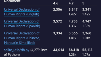
 10
10 0
0- 0


 已为社区贡献3条内容

所有评论(0)