通义千问3-Next-80B-A3B-Instruct：重新定义超长上下文与高效推理的边界

混合注意力机制与高稀疏度MoE架构的完美融合，本文将深入解析阿里云通义千问团队这一革命性模型如何突破传统Transformer的局限，实现超长上下文理解与高效推理的平衡。

一、Qwen3-Next架构核心突破

1.1 混合注意力机制：Gated DeltaNet与Gated Attention的协同创新

Qwen3-Next-80B-A3B的核心架构突破在于其创新的混合注意力设计，将标准注意力机制替换为Gated DeltaNet和Gated Attention的组合。这种设计有效解决了超长上下文序列的计算效率问题，同时保持了强大的建模能力。

Gated DeltaNet基于线性注意力机制，通过状态空间模型(SSM)的方式降低计算复杂度。其数学表达如下：

$$\begin{array}{rl}{h}_t& =\overline{A}{h}_{t-1}+\overline{B}{x}_t\\ y_t& =C{h}_t+D{x}_t\end{array}$$

其中$h_t$是隐藏状态，$x_t$是输入序列，$y_t$是输出序列。$\overline{A}$、$\overline{B}$、$C$、$D$是通过参数化得到的矩阵。这种线性复杂度设计使模型能够高效处理极长序列。

import torch
import torch.nn as nn
import torch.nn.functional as F
from einops import rearrange

class GatedDeltaNet(nn.Module):
    def __init__(self, d_model, num_heads_v=32, num_heads_qk=16, head_dim=128):
        super().__init__()
        self.d_model = d_model
        self.num_heads_v = num_heads_v
        self.num_heads_qk = num_heads_qk
        self.head_dim = head_dim
        
        # 值(value)投影矩阵
        self.W_v = nn.Linear(d_model, num_heads_v * head_dim)
        
        # 查询(Query)和键(Key)投影矩阵
        self.W_qk = nn.Linear(d_model, num_heads_qk * head_dim * 2)
        
        # 输出投影矩阵
        self.W_o = nn.Linear(num_heads_v * head_dim, d_model)
        
        # 门控机制
        self.gate = nn.Linear(d_model, d_model)
        self.gate_act = nn.Sigmoid()
        
        # 状态参数初始化
        self.A = nn.Parameter(torch.randn(num_heads_qk, head_dim, head_dim))
        self.B = nn.Parameter(torch.randn(num_heads_qk, head_dim, head_dim))
        
    def forward(self, x):
        batch_size, seq_len, _ = x.shape
        
        # 值投影和重塑
        V = self.W_v(x)
        V = rearrange(V, 'b s (h d) -> b h s d', h=self.num_heads_v)
        
        # 查询和键投影
        QK = self.W_qk(x)
        QK = rearrange(QK, 'b s (h d two) -> two b h s d', h=self.num_heads_qk, two=2)
        Q, K = QK[0], QK[1]
        
        # 线性注意力计算
        output = self.linear_attention(Q, K, V)
        
        # 输出投影
        output = rearrange(output, 'b h s d -> b s (h d)')
        output = self.W_o(output)
        
        # 门控机制
        gate_value = self.gate_act(self.gate(x))
        output = gate_value * output
        
        return output
    
    def linear_attention(self, Q, K, V):
        # 实现线性注意力计算
        # 简化版实现，实际代码更复杂
        KV = torch.einsum('bhsd,bhse->bhde', K, V)
        Z = 1 / (torch.einsum('bhsd,bhd->bhs', Q, K.sum(dim=2)) + 1e-6)
        output = torch.einsum('bhsd,bhde,bhs->bhse', Q, KV, Z)
        return output

Gated DeltaNet通过线性注意力机制将计算复杂度从二次降为线性，使其能够高效处理长达262K token的序列。门控机制则允许模型动态调整信息流，增强表达能力和训练稳定性。

Gated Attention部分则保留了传统注意力机制的优势，用于捕捉局部依赖关系和精细模式：

class GatedAttention(nn.Module):
    def __init__(self, d_model, num_heads_q=16, num_heads_kv=2, head_dim=256):
        super().__init__()
        self.d_model = d_model
        self.num_heads_q = num_heads_q
        self.num_heads_kv = num_heads_kv
        self.head_dim = head_dim
        
        # 查询投影
        self.W_q = nn.Linear(d_model, num_heads_q * head_dim)
        
        # 键值投影（共享专家）
        self.W_kv = nn.Linear(d_model, num_heads_kv * head_dim * 2)
        
        # 输出投影
        self.W_o = nn.Linear(num_heads_q * head_dim, d_model)
        
        # 门控机制
        self.gate = nn.Linear(d_model, d_model)
        self.gate_act = nn.Sigmoid()
        
        # 旋转位置编码
        self.rotary_emb = RotaryEmbedding(head_dim // 2)  # 64维旋转编码
        
    def forward(self, x, mask=None):
        batch_size, seq_len, _ = x.shape
        
        # 查询投影
        Q = self.W_q(x)
        Q = rearrange(Q, 'b s (h d) -> b h s d', h=self.num_heads_q)
        
        # 键值投影
        KV = self.W_kv(x)
        KV = rearrange(KV, 'b s (h d two) -> two b h s d', h=self.num_heads_kv, two=2)
        K, V = KV[0], KV[1]
        
        # 应用旋转位置编码
        Q = self.rotary_emb(Q, seq_len)
        K = self.rotary_emb(K, seq_len)
        
        # 缩放点积注意力
        scores = torch.matmul(Q, K.transpose(-2, -1)) / math.sqrt(self.head_dim)
        
        if mask is not None:
            scores = scores.masked_fill(mask == 0, -1e9)
        
        attention = torch.softmax(scores, dim=-1)
        output = torch.matmul(attention, V)
        
        # 输出投影
        output = rearrange(output, 'b h s d -> b s (h d)')
        output = self.W_o(output)
        
        # 门控机制
        gate_value = self.gate_act(self.gate(x))
        output = gate_value * output
        
        return output

这种混合设计使模型既能高效处理长序列，又能保持对局部模式的敏感度，在多项基准测试中展现出卓越性能。

1.2 高稀疏度混合专家系统(MoE)：效率与容量的完美平衡

Qwen3-Next-80B-A3B采用了极其稀疏的MoE架构，在总共80B参数中仅激活3B参数（激活率3.75%），大幅降低了计算开销同时保持了模型容量。

class MoEExpert(nn.Module):
    def __init__(self, d_model, d_ff=512):
        super().__init__()
        self.up_proj = nn.Linear(d_model, d_ff)
        self.act = nn.GELU()
        self.down_proj = nn.Linear(d_ff, d_model)
        self.dropout = nn.Dropout(0.1)
        
    def forward(self, x):
        return self.down_proj(self.dropout(self.act(self.up_proj(x))))

class SparseMoELayer(nn.Module):
    def __init__(self, d_model, num_experts=512, num_active_experts=10, d_ff=512):
        super().__init__()
        self.d_model = d_model
        self.num_experts = num_experts
        self.num_active_experts = num_active_experts
        self.d_ff = d_ff
        
        # 专家网络
        self.experts = nn.ModuleList([MoEExpert(d_model, d_ff) for _ in range(num_experts)])
        
        # 门控网络
        self.gate = nn.Linear(d_model, num_experts)
        
        # 共享专家（总是激活）
        self.shared_expert = MoEExpert(d_model, d_ff)
        
    def forward(self, x):
        batch_size, seq_len, _ = x.shape
        
        # 计算门控权重
        gate_logits = self.gate(x)  # [batch_size, seq_len, num_experts]
        gate_weights = F.softmax(gate_logits, dim=-1)
        
        # 选择top-k专家
        topk_weights, topk_indices = torch.topk(
            gate_weights, self.num_active_experts, dim=-1)
        
        # 归一化权重
        topk_weights = topk_weights / (topk_weights.sum(dim=-1, keepdim=True) + 1e-9)
        
        # 初始化输出
        output = torch.zeros_like(x)
        
        # 计算每个token的专家输出
        for i in range(self.num_active_experts):
            # 创建专家掩码
            expert_mask = (topk_indices == i).any(dim=-1)
            
            if expert_mask.any():
                # 获取当前专家处理的token
                expert_input = x[expert_mask]
                
                # 通过专家网络
                expert_output = self.experts[i](expert_input)
                
                # 应用权重
                current_weights = topk_weights[expert_mask, i].unsqueeze(-1)
                expert_output = expert_output * current_weights
                
                # 累加到输出
                output[expert_mask] += expert_output
        
        # 添加共享专家输出
        shared_output = self.shared_expert(x)
        output += shared_output
        
        return output

MoE架构通过动态路由机制，将不同token分配给不同的专家网络处理，实现了计算资源的智能分配。高稀疏度设计（仅激活3.75%的参数）使模型在推理时大幅减少FLOPs，同时保持强大的表达能力。

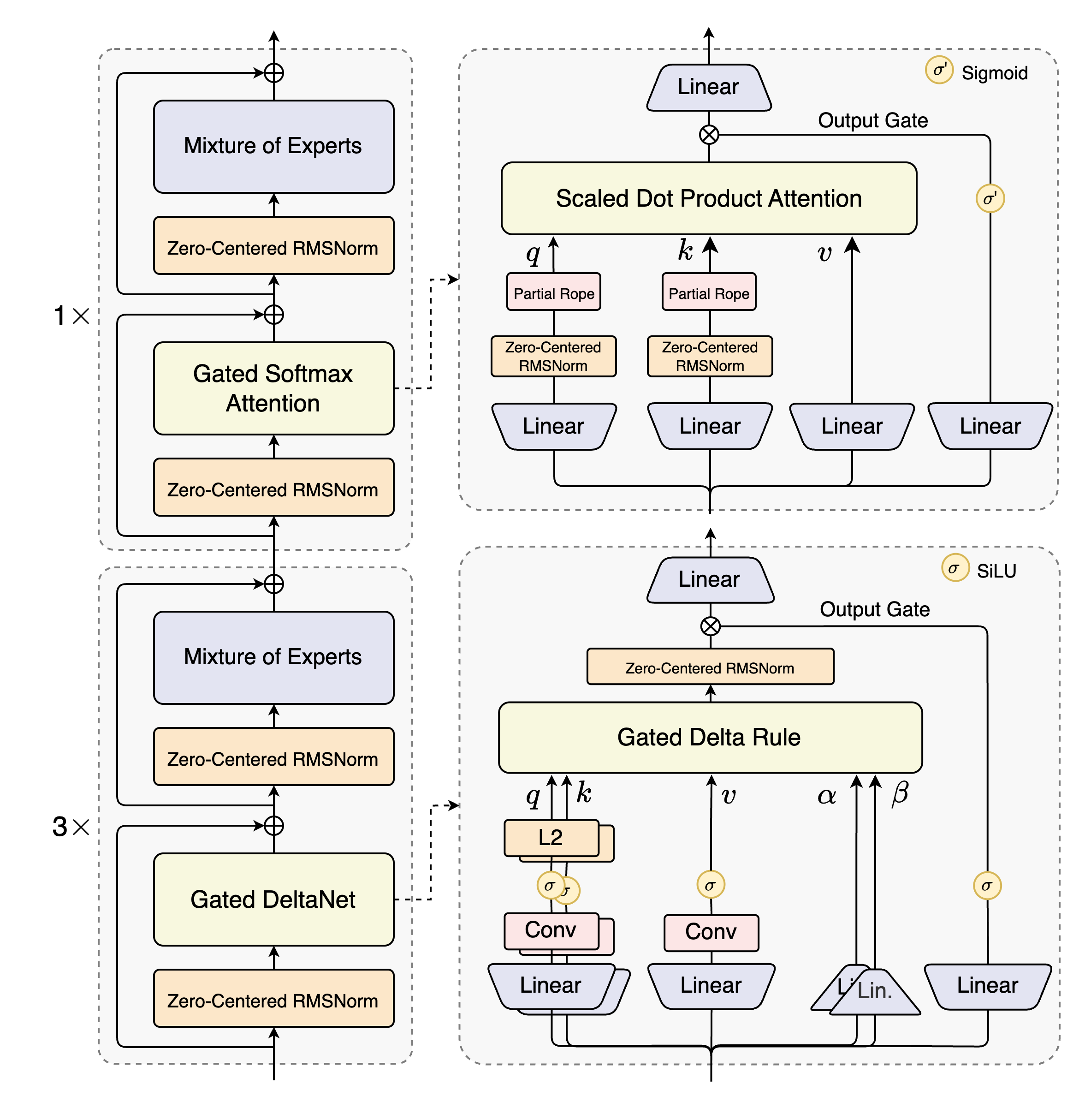
图1：Qwen3-Next设计架构

二、训练技术创新与优化策略

2.1 多令牌预测(MTP)：加速训练与推理的创新方法

多令牌预测是Qwen3-Next的重要创新，通过同时预测多个未来token显著加速训练过程和推理速度。

class MultiTokenPrediction(nn.Module):
    def __init__(self, d_model, vocab_size, num_predict_tokens=4):
        super().__init__()
        self.d_model = d_model
        self.vocab_size = vocab_size
        self.num_predict_tokens = num_predict_tokens
        
        # 多令牌预测头
        self.prediction_heads = nn.ModuleList([
            nn.Linear(d_model, vocab_size) for _ in range(num_predict_tokens)
        ])
        
    def forward(self, hidden_states, labels=None):
        # hidden_states: [batch_size, seq_len, d_model]
        batch_size, seq_len, _ = hidden_states.shape
        
        # 为每个预测位置生成输出
        all_logits = []
        for i in range(self.num_predict_tokens):
            # 选择对应位置的隐藏状态
            # 预测第i个未来token使用第i个隐藏状态
            position_hidden = hidden_states[:, i:seq_len-self.num_predict_tokens+i, :]
            
            # 通过预测头
            logits = self.prediction_heads[i](position_hidden)
            all_logits.append(logits)
        
        if labels is not None:
            # 计算多令牌预测损失
            losses = []
            for i in range(self.num_predict_tokens):
                # 获取对应位置的标签
                position_labels = labels[:, i+1:seq_len-self.num_predict_tokens+i+1]
                
                # 计算交叉熵损失
                loss = F.cross_entropy(
                    all_logits[i].view(-1, self.vocab_size),
                    position_labels.contiguous().view(-1),
                    ignore_index=-100
                )
                losses.append(loss)
            
            # 加权求和损失
            total_loss = sum(loss * (0.8 ** i) for i, loss in enumerate(losses))
            return all_logits, total_loss
        
        return all_logits

# 整合MTP到完整模型
class Qwen3NextWithMTP(nn.Module):
    def __init__(self, config):
        super().__init__()
        self.config = config
        self.transformer = Qwen3NextTransformer(config)
        self.mtp = MultiTokenPrediction(
            config.d_model, config.vocab_size, config.num_predict_tokens
        )
        
    def forward(self, input_ids, labels=None):
        # 获取隐藏状态
        hidden_states = self.transformer(input_ids)
        
        # 多令牌预测
        if labels is not None:
            logits, loss = self.mtp(hidden_states, labels)
            return logits, loss
        else:
            logits = self.mtp(hidden_states)
            return logits

多令牌预测通过同时预测多个未来token，提高了训练样本的效率，加快了模型收敛速度。在推理时，MTP通过推测性解码等技术显著提升生成速度。

2.2 稳定性优化：零中心化与权重衰减层归一化

Qwen3-Next采用了多项稳定性优化技术，确保大规模模型训练的稳定性：

class ZeroCenteredLayerNorm(nn.Module):
    """零中心化层归一化，提高训练稳定性"""
    def __init__(self, normalized_shape, eps=1e-5):
        super().__init__()
        self.eps = eps
        self.normalized_shape = normalized_shape
        
        # 可学习参数
        self.weight = nn.Parameter(torch.ones(normalized_shape))
        self.bias = nn.Parameter(torch.zeros(normalized_shape))
        
    def forward(self, x):
        # 计算均值和方差
        mean = x.mean(dim=-1, keepdim=True)
        var = x.var(dim=-1, keepdim=True, unbiased=False)
        
        # 归一化
        x_normalized = (x - mean) / torch.sqrt(var + self.eps)
        
        # 零中心化变换
        return self.weight * x_normalized + self.bias - self.weight.mean()

class WeightDecayLayerNorm(nn.Module):
    """权重衰减层归一化，防止过拟合"""
    def __init__(self, normalized_shape, eps=1e-5, weight_decay=0.01):
        super().__init__()
        self.eps = eps
        self.normalized_shape = normalized_shape
        self.weight_decay = weight_decay
        
        self.weight = nn.Parameter(torch.ones(normalized_shape))
        self.bias = nn.Parameter(torch.zeros(normalized_shape))
        
    def forward(self, x):
        # 标准层归一化计算
        mean = x.mean(dim=-1, keepdim=True)
        var = x.var(dim=-1, keepdim=True, unbiased=False)
        
        x_normalized = (x - mean) / torch.sqrt(var + self.eps)
        
        # 应用权重衰减正则化
        if self.training:
            # 在训练时应用权重衰减
            self.weight.data = self.weight.data * (1 - self.weight_decay)
        
        return self.weight * x_normalized + self.bias

# 稳定性优化的前馈网络
class StabilizedFeedForward(nn.Module):
    def __init__(self, d_model, d_ff, dropout=0.1):
        super().__init__()
        self.up_proj = nn.Linear(d_model, d_ff)
        self.act = nn.GELU()
        self.down_proj = nn.Linear(d_ff, d_model)
        
        # 使用零中心化层归一化
        self.norm1 = ZeroCenteredLayerNorm(d_model)
        self.norm2 = ZeroCenteredLayerNorm(d_ff)
        
        self.dropout = nn.Dropout(dropout)
        
        # 初始化技巧
        self._init_weights()
        
    def _init_weights(self):
        # 应用特定初始化策略
        nn.init.xavier_uniform_(self.up_proj.weight)
        nn.init.zeros_(self.up_proj.bias)
        
        nn.init.xavier_uniform_(self.down_proj.weight, gain=0.5)  # 减小增益提高稳定性
        nn.init.zeros_(self.down_proj.bias)
        
    def forward(self, x):
        residual = x
        
        # 预归一化
        x = self.norm1(x)
        
        # 上投影和激活
        x = self.up_proj(x)
        x = self.act(x)
        
        # 中间归一化
        x = self.norm2(x)
        
        # 下投影和dropout
        x = self.down_proj(x)
        x = self.dropout(x)
        
        # 残差连接
        return residual + x

这些稳定性优化技术确保了80B参数规模模型的稳定训练，避免了梯度爆炸和数值不稳定问题，为超大规模模型训练提供了重要保障。

三、模型部署与推理优化

3.1 高效推理框架集成：vLLM与SGLang的最佳实践

Qwen3-Next支持多种高效推理框架，以下是使用vLLM进行部署的示例：

# 安装最新vLLM（支持Qwen3-Next）
# pip install vllm --pre --extra-index-url https://wheels.vllm.ai/nightly

from vllm import LLM, SamplingParams
import torch

# 初始化模型（使用ModelScope）
model = LLM(
    model="Qwen/Qwen3-Next-80B-A3B-Instruct",
    tensor_parallel_size=4,  # 4卡张量并行
    max_model_len=262144,    # 支持256K上下文
    trust_remote_code=True,
    dtype="auto",           # 自动选择精度
    gpu_memory_utilization=0.9  # GPU内存利用率
)

# 配置采样参数
sampling_params = SamplingParams(
    temperature=0.7,
    top_p=0.8,
    top_k=20,
    min_p=0.01,            # 最小概率阈值
    max_tokens=16384,      # 最大生成长度
    presence_penalty=0.1,  # 重复惩罚
)

# 准备输入
prompts = [
    "请详细解释量子计算的基本原理及其在人工智能领域的应用前景。",
    "编写一个Python程序，使用PyTorch实现一个简单的Transformer模型。"
]

# 批量推理
outputs = model.generate(prompts, sampling_params)

# 输出结果
for i, output in enumerate(outputs):
    print(f"Prompt {i+1}: {prompts[i]}")
    print(f"Generated: {output.outputs[0].text}")
    print("-" * 50)

对于需要处理超长上下文的场景，可以启用YaRN扩展上下文长度：

# 使用YaRN扩展上下文至1M token
model = LLM(
    model="Qwen/Qwen3-Next-80B-A3B-Instruct",
    tensor_parallel_size=4,
    max_model_len=1010000,  # 扩展至约1M token
    rope_scaling={
        "rope_type": "yarn",
        "factor": 4.0,
        "original_max_position_embeddings": 262144
    },
    swap_space=16,  # GPU-CPU交换空间(GB)
    enforce_eager=True  # 优化长序列性能
)

3.2 SGLang部署与流式响应

SGLang针对Qwen3-Next进行了深度优化，特别适合长上下文和流式响应场景：

import sglang as sgl
from sglang import function, system, user, assistant, gen, set_default_backend

# 设置SGLang后端
@sgl.function
def qwen3_next_chat(s, question):
    s += system("你是一个有帮助的AI助手，请用中文回答用户问题。")
    s += user(question)
    s += assistant(gen("response", max_tokens=16384, temperature=0.7))

# 初始化后端
backend = sgl.OpenAI(
    "http://localhost:30000/v1",  # SGLang服务器地址
    api_key="EMPTY",
    model="Qwen/Qwen3-Next-80B-A3B-Instruct"
)
set_default_backend(backend)

# 流式生成
def stream_chat_response(question):
    state = qwen3_next_chat.run(question, stream=True)
    
    for text in state.text_stream:
        print(text, end="", flush=True)
        # 实际应用中可发送到前端
        yield text
    
    print()  # 换行

# 使用示例
question = "请详细解释混合专家模型(MoE)的工作原理及其在大语言模型中的应用。"
for chunk in stream_chat_response(question):
    # 处理流式输出
    pass

SGLang还支持高级推理优化，如推测性解码和多步推理：

# 启用MTP推测性解码优化
backend = sgl.OpenAI(
    "http://localhost:30000/v1",
    api_key="EMPTY",
    model="Qwen/Qwen3-Next-80B-A3B-Instruct",
    extra_headers={
        "X-Speculative-Algo": "NEXTN",
        "X-Speculative-Num-Steps": "3",
        "X-Speculative-Num-Draft-Tokens": "4"
    }
)

# 复杂推理任务
@sgl.function
def complex_reasoning(s, problem):
    s += system("你是一个数学专家，请逐步解决以下问题并给出最终答案。")
    s += user(problem)
    
    # 分步推理
    with s.user():
        s += "请逐步推理，并将最终答案放在\\boxed{}内。"
    
    with s.assistant():
        s += "让我们逐步分析这个问题：\n"
        s += gen("reasoning", max_tokens=2048, temperature=0.3)
        s += "\n因此，最终答案是：\\boxed{" + gen("answer", max_tokens=10) + "}"

四、代理能力与工具调用

4.1 多工具协同与动态调度

Qwen3-Next在代理能力方面显著提升，支持复杂的多工具协同任务：

from qwen_agent.agents import Assistant
from qwen_agent.tools import BaseTool
import json

# 自定义工具示例
class WeatherTool(BaseTool):
    name = "get_weather"
    description = "获取指定城市的天气信息"
    parameters = {
        "type": "object",
        "properties": {
            "city": {"type": "string", "description": "城市名称"}
        },
        "required": ["city"]
    }
    
    def call(self, city: str):
        # 模拟天气API调用
        # 实际应用中替换为真实API
        weather_data = {
            "city": city,
            "temperature": "22°C",
            "condition": "晴",
            "humidity": "65%",
            "forecast": "未来三天晴朗"
        }
        return json.dumps(weather_data, ensure_ascii=False)

class StockTool(BaseTool):
    name = "get_stock_price"
    description = "获取股票当前价格"
    parameters = {
        "type": "object",
        "properties": {
            "symbol": {"type": "string", "description": "股票代码"}
        },
        "required": ["symbol"]
    }
    
    def call(self, symbol: str):
        # 模拟股票API
        stock_data = {
            "symbol": symbol,
            "price": "156.78",
            "change": "+2.34",
            "change_percent": "+1.52%"
        }
        return json.dumps(stock_data, ensure_ascii=False)

# 初始化代理
llm_cfg = {
    'model': 'Qwen3-Next-80B-A3B-Instruct',
    'model_server': 'http://localhost:8000/v1',
    'api_key': 'EMPTY',
}

tools = [WeatherTool(), StockTool(), 'code_interpreter']

agent = Assistant(llm=llm_cfg, function_list=tools)

# 复杂多工具任务
def execute_complex_task(user_query):
    messages = [{'role': 'user', 'content': user_query}]
    
    print("用户查询:", user_query)
    print("Agent思考中...\n")
    
    for response in agent.run(messages=messages, stream=True):
        if 'content' in response:
            print(response['content'], end='', flush=True)
        elif 'function_call' in response:
            func_call = response['function_call']
            print(f"\n[调用工具: {func_call['name']}]")
            print(f"参数: {func_call['arguments']}")
    
    print("\n\n任务完成")

# 示例查询
complex_query = """
首先获取北京的天气，然后查看苹果公司(AAPL)的股票价格，
最后用Python分析这两个数据之间是否存在相关性，并给出结论。
"""

execute_complex_task(complex_query)

4.2 实时数据处理与可视化

Qwen3-Next强大的代码解释能力支持复杂数据分析和可视化：

import matplotlib.pyplot as plt
import numpy as np
import pandas as pd
from io import BytesIO
import base64

class DataAnalysisTool(BaseTool):
    name = "data_analysis"
    description = "执行数据分析和可视化"
    parameters = {
        "type": "object",
        "properties": {
            "data": {"type": "string", "description": "JSON格式的数据"},
            "analysis_type": {"type": "string", "enum": ["correlation", "trend", "distribution"]},
            "visualization": {"type": "boolean", "description": "是否生成可视化"}
        },
        "required": ["data", "analysis_type"]
    }
    
    def call(self, data: str, analysis_type: str, visualization: bool = True):
        # 解析数据
        df = pd.read_json(data)
        
        result = {"analysis": "", "visualization": None}
        
        if analysis_type == "correlation":
            correlation = df.corr().to_dict()
            result["analysis"] = f"数据相关性分析：\n{json.dumps(correlation, indent=2)}"
            
            if visualization:
                plt.figure(figsize=(10, 8))
                plt.matshow(df.corr(), fignum=1)
                plt.colorbar()
                plt.title('Feature Correlation Matrix')
                
                # 保存为base64
                img_buffer = BytesIO()
                plt.savefig(img_buffer, format='png')
                img_buffer.seek(0)
                result["visualization"] = base64.b64encode(img_buffer.getvalue()).decode('utf-8')
                plt.close()
                
        elif analysis_type == "trend":
            # 趋势分析逻辑
            pass
            
        return json.dumps(result, ensure_ascii=False)

# 集成到代理
tools.append(DataAnalysisTool())
agent = Assistant(llm=llm_cfg, function_list=tools)

五、性能评估与基准测试

5.1 综合能力评估结果

Qwen3-Next-80B-A3B在多项基准测试中表现出色，以下是与前代模型的对比：

模型	MMLU-Pro	GPQA	AIME25	LiveCodeBench	IFEval	Arena-Hard v2
Qwen3-32B	71.9	54.6	20.2	29.1	83.2	34.1
Qwen3-30B-A3B	78.4	70.4	61.3	43.2	84.7	69.0
Qwen3-235B-A22B	83.0	77.5	70.3	51.8	88.7	79.2
Qwen3-Next-80B-A3B	80.6	72.9	69.5	56.6	87.6	82.7

数据显示，Qwen3-Next-80B-A3B在以10%的训练成本下，性能显著超过Qwen3-32B，并在多项测试中接近甚至超越Qwen3-235B-A22B。

5.2 长上下文性能测试

在RULER基准测试中，Qwen3-Next展现出卓越的长上下文理解能力：

# 长上下文性能评估脚本
def evaluate_long_context_performance(model, context_lengths):
    results = {}
    
    for length in context_lengths:
        print(f"测试上下文长度: {length}")
        
        # 生成测试文本
        test_text = generate_long_text(length)
        
        # 准备问题
        questions = generate_questions(test_text, num_questions=5)
        
        accuracy = 0
        for question in questions:
            # 构建完整提示
            prompt = f"文本：{test_text}\n\n问题：{question}\n\n答案："
            
            # 获取模型回答
            response = model.generate(prompt, max_length=length+100)
            
            # 评估答案正确性
            if evaluate_answer(response, question):
                accuracy += 1
        
        results[length] = accuracy / len(questions)
        print(f"长度 {length} 准确率: {results[length]:.3f}")
    
    return results

# 测试不同上下文长度
context_lengths = [4096, 8192, 16384, 32768, 65536, 131072, 262144]
performance_results = evaluate_long_context_performance(model, context_lengths)

# 可视化结果
plt.plot(list(performance_results.keys()), list(performance_results.values()))
plt.xlabel('Context Length')
plt.ylabel('Accuracy')
plt.title('Long Context Performance')
plt.show()

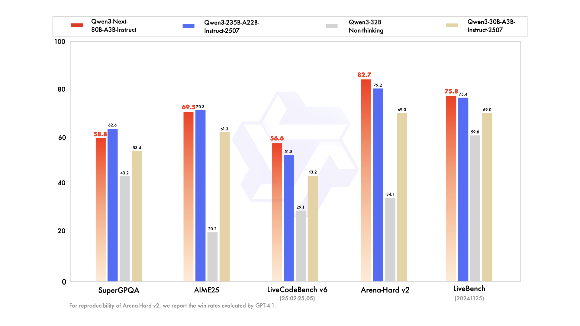
图2：Qwen3-Next在不同上下文长度下的性能表现（来源：RULER基准测试）

六、未来发展方向与应用前景

6.1 多模态融合与跨模态理解

Qwen3-Next为多模态应用奠定了坚实基础，未来的扩展可能包括：

class MultiModalQwen3Next(nn.Module):
    def __init__(self, config):
        super().__init__()
        self.text_encoder = Qwen3NextTransformer(config)
        self.vision_encoder = VisionTransformer(config.vision_config)
        self.fusion_module = CrossModalAttention(config)
        
    def forward(self, text_input, image_input):
        text_features = self.text_encoder(text_input)
        image_features = self.vision_encoder(image_input)
        
        # 跨模态注意力融合
        fused_features = self.fusion_module(text_features, image_features)
        
        return fused_features

# 多模态应用示例
def multimodal_qa(text_question, image):
    # 编码文本和图像
    text_emb = model.text_encoder.encode(text_question)
    image_emb = model.vision_encoder.encode(image)
    
    # 多模态融合
    multimodal_emb = model.fusion_module(text_emb, image_emb)
    
    # 生成答案
    answer = model.decoder.generate(multimodal_emb)
    
    return answer

6.2 自适应计算与动态架构

未来版本可能引入更灵活的动态架构：

class AdaptiveComputationModel(nn.Module):
    def __init__(self, config):
        super().__init__()
        self.config = config
        self.layers = nn.ModuleList([AdaptiveLayer(config) for _ in range(config.num_layers)])
        self.routing_network = RoutingNetwork(config)
        
    def forward(self, x, complexity_threshold=0.5):
        # 根据输入复杂度动态选择计算路径
        routing_weights = self.routing_network(x)
        
        for i, layer in enumerate(self.layers):
            # 决定是否跳过该层或使用简化计算
            if routing_weights[i] < complexity_threshold:
                continue
                
            # 动态选择专家或计算模式
            computation_mode = self.select_computation_mode(x, i)
            x = layer(x, mode=computation_mode)
        
        return x

结论：通向高效通用人工智能的新里程碑

Qwen3-Next-80B-A3B-Instruct代表了大规模语言模型发展的重要里程碑，通过混合注意力机制、高稀疏度MoE架构和多令牌预测等创新技术，实现了效率与性能的突破性平衡。

核心贡献总结：

1. 架构创新：Gated DeltaNet + Gated Attention混合设计，高效处理超长序列
2. 稀疏高效：3.75%激活率的MoE架构，大幅降低计算成本
3. 训练优化：多令牌预测加速训练，稳定性技术确保大规模训练可靠性
4. 长上下文：原生支持256K上下文，可扩展至1M token
5. 代理能力：强大的工具调用和多步推理能力

Qwen3-Next不仅在多项基准测试中展现卓越性能，更在实际应用中提供了可行的部署方案，为下一代AI应用奠定了坚实基础。随着多模态扩展和自适应计算等方向的进一步发展，Qwen3-Next架构将继续引领高效通用人工智能的前沿探索。

---

参考资源：

1. Qwen3-Next Technical Report (Qwen3-Next技术报告)
2. ModelScope模型库
3. vLLM高效推理框架
4. SGLang流式处理框架
5. Qwen-Agent工具调用库