图解Word2Vec:如何让AI真正“读懂”人类语言?
定义 Skip-Gram 类import torch.nn as nn # 导入 neural network# 从词汇表大小到嵌入层大小(维度)的线性层(权重矩阵)# 从嵌入层大小(维度)到词汇表大小的线性层(权重矩阵)def forward(self, X): # 前向传播的方式,X 形状为 (batch_size, voc_size)# 通过隐藏层,hidden 形状为 (batch_siz
图解Word2Vec:如何让AI真正“读懂”人类语言?
一、从"文字游戏"到"语义地图":词向量革命
“国王 - 男人 + 女人 = 女王”
这个震撼NLP界的经典公式,揭开了词向量的神秘面纱
传统文本处理就像让AI玩"文字连连看":机械统计词频、匹配固定规则。这种处理方式最大的痛点是什么?看看这个例子:
病例报告
患者:“医生,我最近总是心慌、手抖、容易饿”
传统AI诊断:发现"心"出现3次,"手"出现2次 → 重点检查心血管系统
实际诊断:甲状腺功能亢进
这个真实的医疗AI误诊案例,暴露了传统文本处理的致命缺陷——只见树木不见森林。而词向量的诞生,让AI第一次拥有了理解词语深层含义的能力。
二、Word2Vec的魔法原理(附代码实战)
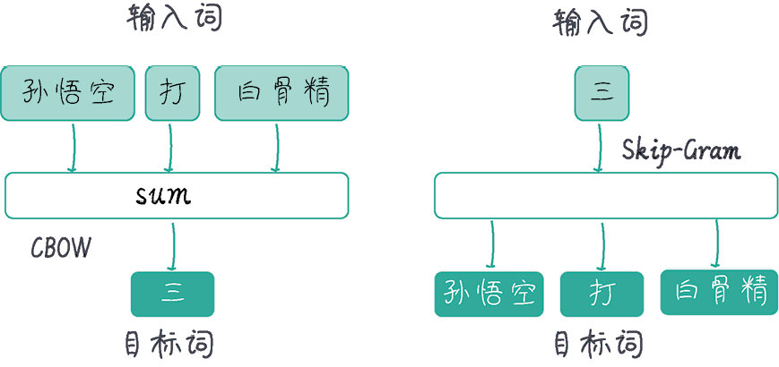
2.1 从"填空题"到"完形填空":两大核心模型
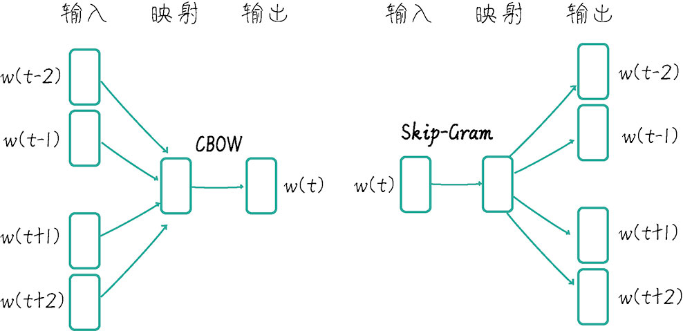
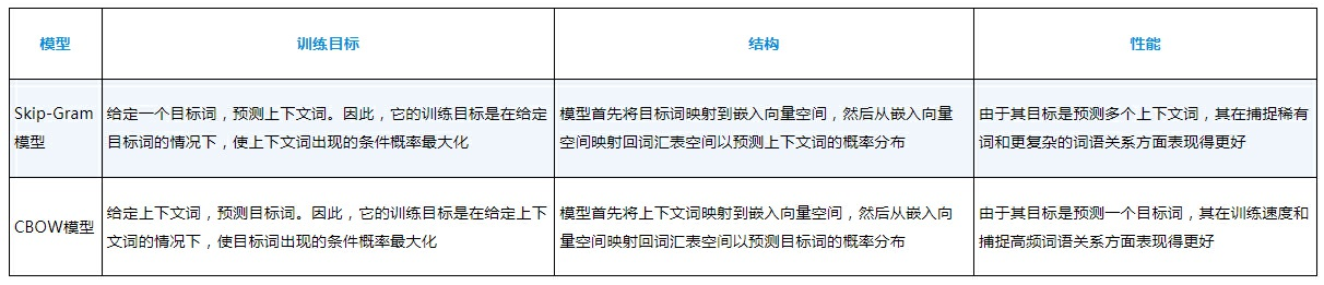
- CBOW模型:像做填空题
输入:四周的词语(如"猫 会 __ 老鼠")
输出:预测中间词(“抓”) - Skip-Gram模型:像完形填空
输入:中心词(如"人工智能")
输出:预测周围词(“深度学习”、“算法”、“大数据”)
2.2 Skip-Gram模型的代码实现
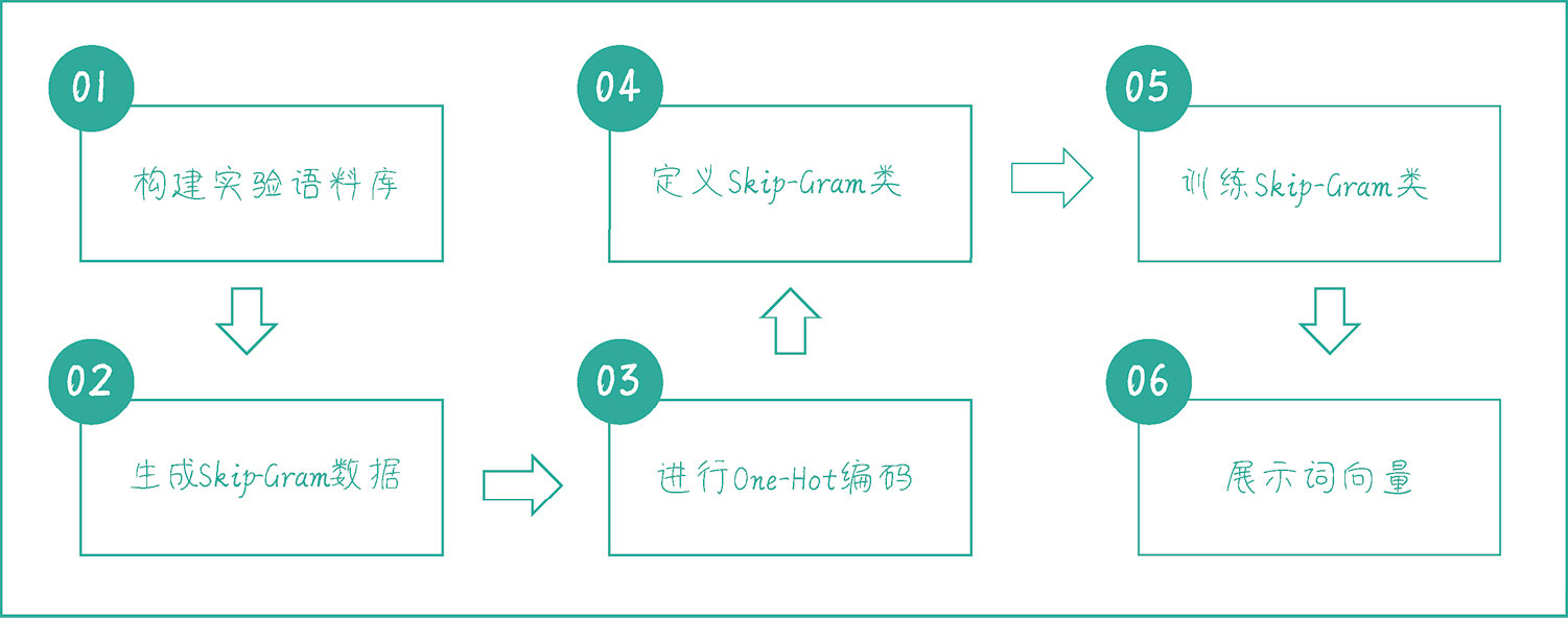
2.2.1 构建实验语料库
# 定义一个句子列表,后面会用这些句子来训练 CBOW 和 Skip-Gram 模型
sentences = ["Kage is Teacher", "Mazong is Boss", "Niuzong is Boss",
             "Xiaobing is Student", "Xiaoxue is Student",]
# 将所有句子连接在一起,然后用空格分隔成多个单词
words = ' '.join(sentences).split()
# 构建词汇表,去除重复的词
word_list = list(set(words))
# 创建一个字典,将每个词映射到一个唯一的索引
word_to_idx = {word: idx for idx, word in enumerate(word_list)}
# 创建一个字典,将每个索引映射到对应的词
idx_to_word = {idx: word for idx, word in enumerate(word_list)}
voc_size = len(word_list) # 计算词汇表的大小
print(" 词汇表:", word_list) # 输出词汇表
print(" 词汇到索引的字典:", word_to_idx) # 输出词汇到索引的字典
print(" 索引到词汇的字典:", idx_to_word) # 输出索引到词汇的字典
print(" 词汇表大小:", voc_size) # 输出词汇表大小
 词汇表: ['Xiaoxue', 'is', 'Niuzong', 'Student', 'Teacher', 'Boss', 'Mazong', 'Xiaobing', 'Kage']

 词汇到索引的字典: {'Xiaoxue': 0, 'is': 1, 'Niuzong': 2, 'Student': 3, 'Teacher': 4, 'Boss': 5, 'Mazong': 6, 'Xiaobing': 7, 'Kage': 8}

 索引到词汇的字典: {0: 'Xiaoxue', 1: 'is', 2: 'Niuzong', 3: 'Student', 4: 'Teacher', 5: 'Boss', 6: 'Mazong', 7: 'Xiaobing', 8: 'Kage'}

 词汇表大小: 9
2.2.2 生成Skip-Gram数据
# 生成 Skip-Gram 训练数据
def create_skipgram_dataset(sentences, window_size=2):
    data = [] # 初始化数据
    for sentence in sentences: # 遍历句子
        sentence = sentence.split()  # 将句子分割成单词列表
        for idx, word in enumerate(sentence):  # 遍历单词及其索引
            # 获取相邻的单词,将当前单词前后各 N 个单词作为相邻单词
            for neighbor in sentence[max(idx - window_size, 0):
                        min(idx + window_size + 1, len(sentence))]:
                if neighbor != word:  # 排除当前单词本身
                    # 将相邻单词与当前单词作为一组训练数据
                    data.append((neighbor, word))
    return data
# 使用函数创建 Skip-Gram 训练数据
skipgram_data = create_skipgram_dataset(sentences)
# 打印未编码的 Skip-Gram 数据样例(前 3 个)
print("Skip-Gram 数据样例(未编码):", skipgram_data[:3])
Skip-Gram 数据样例(未编码): [('is', 'Kage'), ('Teacher', 'Kage'), ('Kage', 'is')]
2.2.3 进行One-Hot编码
# 定义 One-Hot 编码函数
import torch # 导入 torch 库
def one_hot_encoding(word, word_to_idx):
    tensor = torch.zeros(len(word_to_idx)) # 创建一个长度与词汇表相同的全 0 张量
    tensor[word_to_idx[word]] = 1  # 将对应词的索引设为 1
    return tensor  # 返回生成的 One-Hot 向量
# 展示 One-Hot 编码前后的数据
word_example = "Teacher"
print("One-Hot 编码前的单词:", word_example)
print("One-Hot 编码后的向量:", one_hot_encoding(word_example, word_to_idx))
# 展示编码后的 Skip-Gram 训练数据样例
print("Skip-Gram 数据样例(已编码):", [(one_hot_encoding(context, word_to_idx),
          word_to_idx[target]) for context, target in skipgram_data[:3]])
One-Hot 编码前的单词: Teacher
One-Hot 编码后的向量: tensor([0., 0., 0., 1., 0., 0., 0., 0., 0.])
Skip-Gram 数据样例(已编码):
[(tensor([0., 0., 0., 0., 1., 0., 0., 0., 0.]), 7), (tensor([0., 0., 0., 1., 0., 0., 0., 0., 0.]), 7), (tensor([0., 0., 0., 0., 0., 0., 0., 1., 0.]), 4)]
2.2.4 定义Skip-Gram类
# 定义 Skip-Gram 类
import torch.nn as nn # 导入 neural network
class SkipGram(nn.Module):
    def __init__(self, voc_size, embedding_size):
        super(SkipGram, self).__init__()
        # 从词汇表大小到嵌入层大小(维度)的线性层(权重矩阵)
        self.input_to_hidden = nn.Linear(voc_size, embedding_size, bias=False)
        # 从嵌入层大小(维度)到词汇表大小的线性层(权重矩阵)
        self.hidden_to_output = nn.Linear(embedding_size, voc_size, bias=False)
    def forward(self, X): # 前向传播的方式,X 形状为 (batch_size, voc_size)
         # 通过隐藏层,hidden 形状为 (batch_size, embedding_size)
            hidden = self.input_to_hidden(X)
            # 通过输出层,output_layer 形状为 (batch_size, voc_size)
            output = self.hidden_to_output(hidden)
            return output
embedding_size = 2 # 设定嵌入层的大小,这里选择 2 是为了方便展示
skipgram_model = SkipGram(voc_size, embedding_size)  # 实例化 Skip-Gram 模型
print("Skip-Gram 模型:", skipgram_model)
Skip-Gram 模型: SkipGram(
  (input_to_hidden): Linear(in_features=9, out_features=2, bias=False)
  (hidden_to_output): Linear(in_features=2, out_features=9, bias=False)
)
2.2.5 训练Skip-Gram
# 训练 Skip-Gram 类
learning_rate = 0.001 # 设置学习速率
epochs = 1000 # 设置训练轮次
criterion = nn.CrossEntropyLoss() # 定义交叉熵损失函数
import torch.optim as optim # 导入随机梯度下降优化器
optimizer = optim.SGD(skipgram_model.parameters(), lr=learning_rate)
# 开始训练循环
loss_values = [] # 用于存储每轮的平均损失值
for epoch in range(epochs):
loss_sum = 0 # 初始化损失值
for context, target in skipgram_data:
X = one_hot_encoding(target, word_to_idx).float().unsqueeze(0) # 将中心词转换为 One-Hot 向量
y_true = torch.tensor([word_to_idx[context]], dtype=torch.long) # 将周围词转换为索引值
y_pred = skipgram_model(X) # 计算预测值
loss = criterion(y_pred, y_true) # 计算损失
loss_sum += loss.item() # 累积损失
optimizer.zero_grad() # 清空梯度
loss.backward() # 反向传播
optimizer.step() # 更新参数
if (epoch+1) % 100 == 0: # 输出每 100 轮的损失,并记录损失
print(f"Epoch: {epoch+1}, Loss: {loss_sum/len(skipgram_data)}")
loss_values.append(loss_sum / len(skipgram_data))
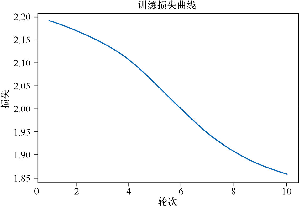
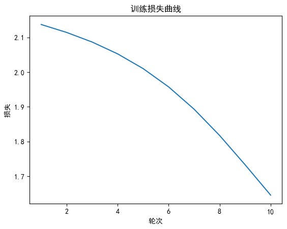
# 绘制训练损失曲线
import matplotlib.pyplot as plt # 导入 matplotlib
# 绘制二维词向量图
plt.rcParams["font.family"]=['SimHei'] # 用来设定字体样式
plt.rcParams['font.sans-serif']=['SimHei'] # 用来设定无衬线字体样式
plt.rcParams['axes.unicode_minus']=False # 用来正常显示负号
plt.plot(range(1, epochs//100 + 1), loss_values) # 绘图
plt.title(' 训练损失曲线 ') # 图题
plt.xlabel(' 轮次 ') # X 轴 Label
plt.ylabel(' 损失 ') # Y 轴 Label
plt.show() # 显示图
Epoch: 100, Loss: 2.176283597946167
Epoch: 200, Loss: 2.1313777963320413
Epoch: 300, Loss: 2.079272961616516
Epoch: 400, Loss: 2.0179983615875243
Epoch: 500, Loss: 1.956022528807322
Epoch: 600, Loss: 1.9065291663010915
Epoch: 700, Loss: 1.8729750255743662
Epoch: 800, Loss: 1.8494429806868236
Epoch: 900, Loss: 1.8303062697251637
Epoch: 1000, Loss: 1.812800904115041
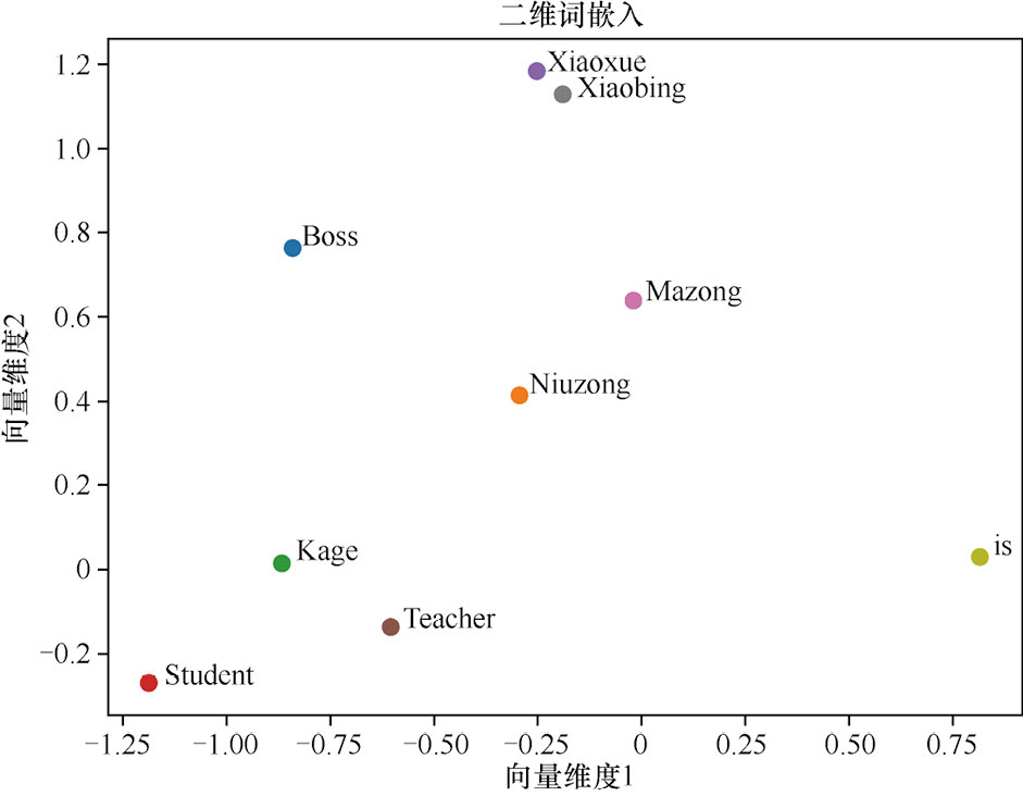
2.2.6 展示词向量
# 输出 Skip-Gram 习得的词嵌入
print("Skip-Gram 词嵌入:")
for word, idx in word_to_idx.items(): # 输出每个词的嵌入向量
 print(f"{word}: {skipgram_model.input_to_hidden.weight[:,idx].detach().numpy()}")
Xiaobing: [-1.3628563 -2.1293848]
Xiaoxue: [-1.3693085 -2.1389563]
Boss: [ 2.923863 -0.4184679]
Student: [-0.09255204 -0.8242733 ]
is: [-0.23261149 0.29151806]
Kage: [-0.3542828 -0.9870443]
Niuzong: [ 0.8161409 -0.624454 ]
Mazong: [ 0.821509 -0.62387395]
Teacher: [ 0.8520589 -0.47847477]
fig, ax = plt.subplots()
for word, idx in word_to_idx.items():
    # 获取每个单词的嵌入向量
    vec = skipgram_model.input_to_hidden.weight[:,idx].detach().numpy()
    ax.scatter(vec[0], vec[1]) # 在图中绘制嵌入向量的点
    ax.annotate(word, (vec[0], vec[1]), fontsize=12) # 点旁添加单词标签
plt.title(' 二维词嵌入 ') # 图题
plt.xlabel(' 向量维度 1') # X 轴 Label
plt.ylabel(' 向量维度 2') # Y 轴 Label
plt.show() # 显示图
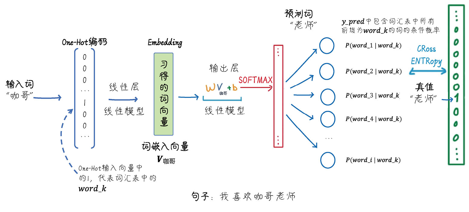
总结⼀下:我们使⽤PyTorch实现了⼀个简单的Word2Vec(这⾥是Skip-Gram)模型。
模型包括输⼊层、隐藏层和输出层。输⼊层接收周围词(以One-Hot编码后的向量形式表示)。接下来,输⼊层到隐藏层的权重矩阵(记为input_to_hidden)将这个向量转换为词嵌⼊,该词嵌⼊直接作为隐藏层的输出。
隐藏层到输出层的权重矩阵(记为hidden_to_output)将隐藏层的
输出转换为⼀个概率分布,⽤于预测与周围词相关的中⼼词(以索引形式表示)。通过最⼩化预测词和实际⽬标词之间的分类交叉熵损失,可以学习词嵌⼊向量。下图展示了这个流程。
2.3 CBOW模型的代码实现
CBOW模型与Skip-Gram模型相反,其主要任务是根据给定的周围词来预测中⼼词。
# 定义一个句子列表,后面会用这些句子来训练 CBOW 和 Skip-Gram 模型
sentences = ["Kage is Teacher", "Mazong is Boss", "Niuzong is Boss",
             "Xiaobing is Student", "Xiaoxue is Student",]
# 将所有句子连接在一起,然后用空格分隔成多个单词
words = ' '.join(sentences).split()
# 构建词汇表,去除重复的词
word_list = list(set(words))
# 创建一个字典,将每个词映射到一个唯一的索引
word_to_idx = {word: idx for idx, word in enumerate(word_list)}
# 创建一个字典,将每个索引映射到对应的词
idx_to_word = {idx: word for idx, word in enumerate(word_list)}
voc_size = len(word_list) # 计算词汇表的大小
print(" 词汇表:", word_list) # 输出词汇表
print(" 词汇到索引的字典:", word_to_idx) # 输出词汇到索引的字典
print(" 索引到词汇的字典:", idx_to_word) # 输出索引到词汇的字典
print(" 词汇表大小:", voc_size) # 输出词汇表大小
 词汇表: ['Boss', 'Niuzong', 'Mazong', 'Teacher', 'is', 'Xiaobing', 'Student', 'Kage', 'Xiaoxue']
 词汇到索引的字典: {'Boss': 0, 'Niuzong': 1, 'Mazong': 2, 'Teacher': 3, 'is': 4, 'Xiaobing': 5, 'Student': 6, 'Kage': 7, 'Xiaoxue': 8}
 索引到词汇的字典: {0: 'Boss', 1: 'Niuzong', 2: 'Mazong', 3: 'Teacher', 4: 'is', 5: 'Xiaobing', 6: 'Student', 7: 'Kage', 8: 'Xiaoxue'}
 词汇表大小: 9
# 生成 CBOW 训练数据
def create_cbow_dataset(sentences, window_size=2):
    data = []# 初始化数据
    for sentence in sentences:
        sentence = sentence.split()  # 将句子分割成单词列表
        for idx, word in enumerate(sentence):  # 遍历单词及其索引
            # 获取上下文词汇,将当前单词前后各 window_size 个单词作为周围词
            context_words = sentence[max(idx - window_size, 0):idx] \
                + sentence[idx + 1:min(idx + window_size + 1, len(sentence))]
            # 将当前单词与上下文词汇作为一组训练数据
            data.append((word, context_words))
    return data
# 使用函数创建 CBOW 训练数据
cbow_data = create_cbow_dataset(sentences)
# 打印未编码的 CBOW 数据样例(前三个)
print("CBOW 数据样例(未编码):", cbow_data[:3])
CBOW 数据样例(未编码): [('Kage', ['is', 'Teacher']), ('is', ['Kage', 'Teacher']), ('Teacher', ['Kage', 'is'])]
# 定义 One-Hot 编码函数
import torch # 导入 torch 库
def one_hot_encoding(word, word_to_idx):
    tensor = torch.zeros(len(word_to_idx)) # 创建一个长度与词汇表相同的全 0 张量
    tensor[word_to_idx[word]] = 1  # 将对应词的索引设为 1
    return tensor  # 返回生成的 One-Hot 向量
# 展示 One-Hot 编码前后的数据
word_example = "Teacher"
print("One-Hot 编码前的单词:", word_example)
print("One-Hot 编码后的向量:", one_hot_encoding(word_example, word_to_idx))
One-Hot 编码前的单词: Teacher
One-Hot 编码后的向量: tensor([0., 0., 0., 1., 0., 0., 0., 0., 0.])
# 定义 CBOW 模型
import torch.nn as nn # 导入 neural network
class CBOW(nn.Module):
    def __init__(self, voc_size, embedding_size):
        super(CBOW, self).__init__()
        # 从词汇表大小到嵌入大小的线性层(权重矩阵)
        self.input_to_hidden = nn.Linear(voc_size,
                                         embedding_size, bias=False)
        # 从嵌入大小到词汇表大小的线性层(权重矩阵)
        self.hidden_to_output = nn.Linear(embedding_size,
                                          voc_size, bias=False)
    def forward(self, X): # X: [num_context_words, voc_size]
        # 生成嵌入:[num_context_words, embedding_size]
        embeddings = self.input_to_hidden(X)
        # 计算隐藏层,求嵌入的均值:[embedding_size]
        hidden_layer = torch.mean(embeddings, dim=0)
        # 生成输出层:[1, voc_size]
        output_layer = self.hidden_to_output(hidden_layer.unsqueeze(0))
        return output_layer
embedding_size = 2 # 设定嵌入层的大小,这里选择 2 是为了方便展示
cbow_model = CBOW(voc_size,embedding_size)  # 实例化 CBOW 模型
print("CBOW 模型:", cbow_model)
CBOW 模型: CBOW(
  (input_to_hidden): Linear(in_features=9, out_features=2, bias=False)
  (hidden_to_output): Linear(in_features=2, out_features=9, bias=False)
)
# 训练 Skip-Gram 类
learning_rate = 0.001 # 设置学习速率
epochs = 1000 # 设置训练轮次
criterion = nn.CrossEntropyLoss()  # 定义交叉熵损失函数
import torch.optim as optim # 导入随机梯度下降优化器
optimizer = optim.SGD(cbow_model.parameters(), lr=learning_rate)
# 开始训练循环
loss_values = []  # 用于存储每轮的平均损失值
for epoch in range(epochs):
    loss_sum = 0 # 初始化损失值
    for target, context_words in cbow_data:
        # 将上下文词转换为 One-Hot 向量并堆叠
        X = torch.stack([one_hot_encoding(word, word_to_idx) for word in context_words]).float()
        # 将目标词转换为索引值
        y_true = torch.tensor([word_to_idx[target]], dtype=torch.long)
        y_pred = cbow_model(X)  # 计算预测值
        loss = criterion(y_pred, y_true)  # 计算损失
        loss_sum += loss.item() # 累积损失
        optimizer.zero_grad()  # 清空梯度
        loss.backward()  # 反向传播
        optimizer.step()  # 更新参数
    if (epoch+1) % 100 == 0: # 输出每 100 轮的损失,并记录损失
      print(f"Epoch: {epoch+1}, Loss: {loss_sum/len(cbow_data)}")
      loss_values.append(loss_sum / len(cbow_data))
# 绘制训练损失曲线
import matplotlib.pyplot as plt # 导入 matplotlib
# 绘制二维词向量图
plt.rcParams["font.family"]=['SimHei'] # 用来设定字体样式
plt.rcParams['font.sans-serif']=['SimHei'] # 用来设定无衬线字体样式
plt.rcParams['axes.unicode_minus']=False # 用来正常显示负号
plt.plot(range(1, epochs//100 + 1), loss_values) # 绘图
plt.title(' 训练损失曲线 ') # 图题
plt.xlabel(' 轮次 ') # X 轴 Label
plt.ylabel(' 损失 ') # Y 轴 Label
plt.show() # 显示图
Epoch: 100, Loss: 2.1371095180511475
Epoch: 200, Loss: 2.114210780461629
Epoch: 300, Loss: 2.0865681091944377
Epoch: 400, Loss: 2.0524648745854694
Epoch: 500, Loss: 2.010000443458557
Epoch: 600, Loss: 1.9573023001352945
Epoch: 700, Loss: 1.893039353688558
Epoch: 800, Loss: 1.817344347635905
Epoch: 900, Loss: 1.7329498807589212
Epoch: 1000, Loss: 1.6456005891164145
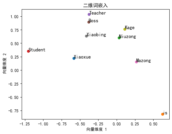
# 输出 Skip-Gram 习得的词嵌入
print("Skip-Gram 词嵌入:")
for word, idx in word_to_idx.items(): # 输出每个词的嵌入向量
 print(f"{word}: {cbow_model.input_to_hidden.weight[:,idx].detach().numpy()}")
Skip-Gram 词嵌入:

Xiaoxue: [-0.5842088   0.21841691]
is: [ 0.6250008 -0.8186659]
Niuzong: [0.03038938 0.60383385]
Student: [-1.2024668  0.3539113]
Teacher: [-0.37656686  1.0371245 ]
Boss: [-0.3826948   0.89280415]
Mazong: [0.2657739  0.15451309]
Xiaobing: [-0.4118811  0.6344902]
Kage: [0.10943636 0.7646477 ]
三、通向AGI的基石:词向量的未来演进
当GPT-4的1536维词向量遇上多模态学习:
- 图像向量:"猫"的向量同时关联图片、叫声、触感
- 跨语言向量:中文"龙"与英文"dragon"的语义差异精准呈现
- 时空向量:"元宇宙"在不同时期的含义演变轨迹
技术演进路线: 传统词向量 → 语境化词向量(ELMo) → 预训练语言模型(BERT/GPT) → 多模态向量

欢迎加入DeepSeek 技术社区。在这里,你可以找到志同道合的朋友,共同探索AI技术的奥秘。
更多推荐


 22
22 0
0- 0


 已为社区贡献2条内容

所有评论(0)