【DeepSeek-R1背后的技术】系列博文：
第1篇：混合专家模型（MoE）
第2篇：大模型知识蒸馏（Knowledge Distillation）
第3篇：强化学习（Reinforcement Learning, RL）
第4篇：本地部署DeepSeek，断网也能畅聊！
第5篇：DeepSeek-R1微调指南
第6篇：思维链（CoT）
第7篇：冷启动
第8篇：位置编码介绍（绝对位置编码、RoPE、ALiBi、YaRN）
第9篇：MLA（Multi-Head Latent Attention，多头潜在注意力）
第10篇：PEFT（参数高效微调——Adapter、Prefix Tuning、LoRA）
第11篇：RAG原理介绍和本地部署（DeepSeek+RAGFlow构建个人知识库）
第12篇：分词算法Tokenizer（WordPiece，Byte-Pair Encoding (BPE)，Byte-level BPE(BBPE)）
第13篇：归一化方式介绍（BatchNorm, LayerNorm, Instance Norm 和 GroupNorm）
第14篇：MoE源码分析（腾讯Hunyuan大模型介绍）

因为DeepSeek-R1没有公布模型框架的源码，我们参考腾讯开源的混元大模型进行代码分析，整体构建上应该和DeepSeek-R1差不多，可能细节上会有些不同。

混元大模型的代码其实和其他MoE模型差不多，结构比较清晰，非常适合上手。

我们先简要介绍一下混元大模型，然后再进行MoE相关的源码分析，如果对Hunyuan大模型不感兴趣的可以直接跳到第三部分内容。

1 混元简介

腾讯的Hunyuan团队开源了一款名为Hunyuan-Large的大模型，是基于Transformer的Mixture of Experts（MoE）模型，拥有3890亿参数和52亿激活参数，能够处理256K的token，它在多个基准测试中表现出色，包括语言理解和生成、逻辑推理、数学问题解决、编程、长文本处理和聚合任务等。其特点如下：

• 大规模合成数据：Hunyuan-Large在预训练阶段使用了比以往文献中更大的合成数据集，这有助于模型学习更丰富的表示，并更好地泛化到未见过的数据。
• 混合专家路由策略：模型采用了共享专家和专门专家的混合路由策略，以及创新的回收路由方法，以提高训练效率和模型性能。
• 关键值缓存压缩技术：通过关键值（KV）缓存压缩技术，Hunyuan-Large显著降低了内存压力，提高了推理效率。
• 专家特定学习率策略：模型为不同专家设置了特定的学习率，优化了训练过程。

相关链接：

GitHub
HuggingFace
论文
官网
API

2 模型介绍

我们先简要介绍一下Hunyuan大模型的数据、模型结构和训练。

2.1 预训练

2.1.1 数据

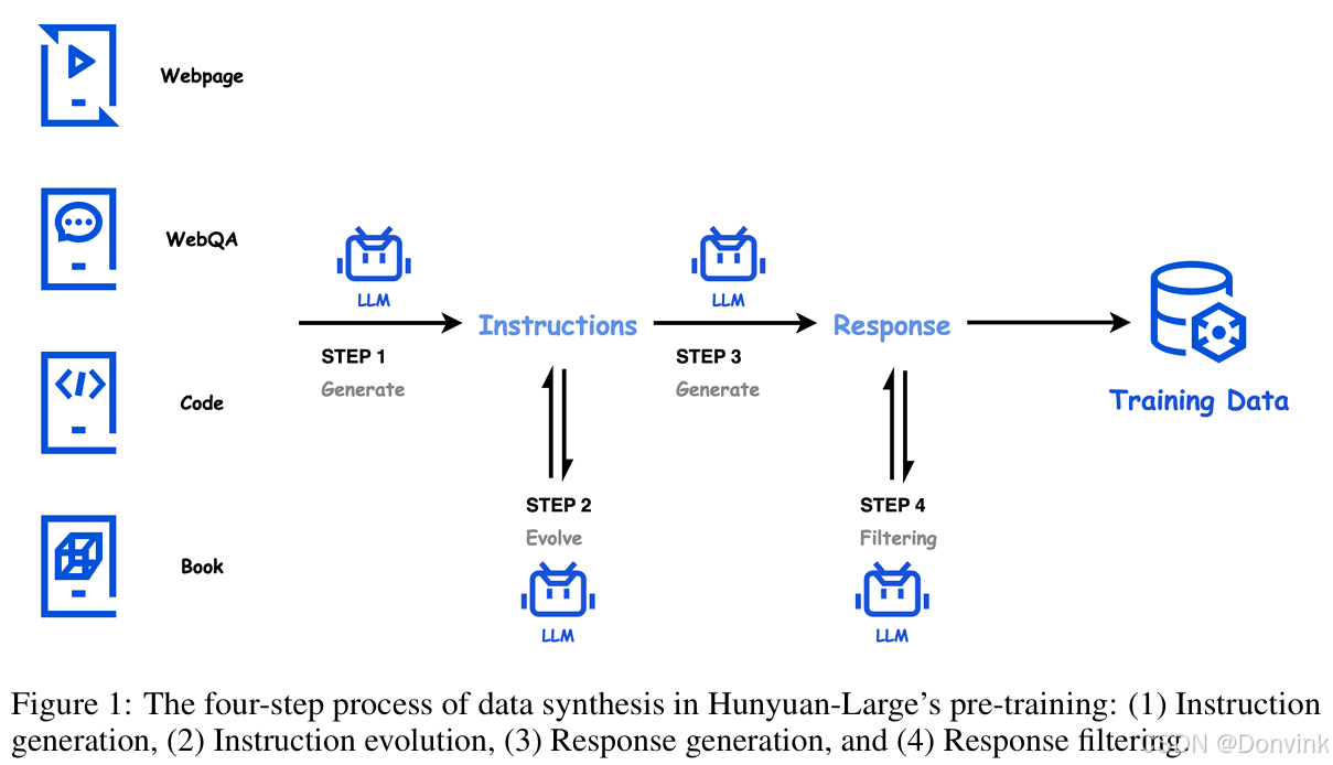
数据处理流程主要包括四步：

• 步骤1：指令生成。为了确保指令的多样性，作者使用高质量、知识丰富的数据源，如网页、基于Web的问答数据、代码库、书籍和其他资源作为种子。这些种子与不同的指令生成提示相配合，能够生成覆盖不同领域的各种指令，这些指令具有不同的期望指令风格和复杂度。

• 步骤2：指令进化。为了进一步改善这些初步指示的质量，按以下三项指引加以改善：(a) 提高指示的清晰度和资料的丰富程度。(b) 通过自我指导增强扩展低资源域指令。© 改进指令以增加其难度级别。这些不断发展的高质量和挑战性指令使模型能够更有效地从合成数据中获益，从而跨越原始的能力界限。

• 步骤3：响应生成。利用几个专门的模型来为上述进化的指令生成信息丰富和准确的答案。这些模型大小不一，并且是精心设计的专用模型，用于合成针对各个领域中的指令的专家级响应。

• 步骤4：响应过滤。为了过滤合成的解释-响应对，作者采用了一个批判模型进行自我一致性检查，其中作者生成多个答案，以执行任务，如客观问答任务的自我一致性过滤，确保可靠性和准确性。这个过程能够有效地删除任何低质量或不一致的数据，确保在预训练中利用高质量的文本。

2.1.2 Tokenizer

分词器是预训练中至关重要的一部分，它需要平衡两个关键因素：

• 实现高压缩率以实现高效的训练和推理，
• 维持一个足够大的词汇量，以确保每个词嵌入都能得到充分学习。

Hunyuan-Large模型采用了一个包含128K个标记的词汇表。这个词汇表是由tiktoken分词器（OpenAI, 2023）中的100K个tokens和额外专门设计用于增强中文支持的28K个tokens组合而成。值得注意的是，与LLama3.1分词器相比，Hunyuan的新分词器提升了压缩率，从2.78个字符增加到3.13个字符每token。

2.2 模型结构

Hunyuan-Large的模型结构主要使用经典的混合专家（MoE, Mixture of Experts）架构，该架构利用多个专家替换了Transformer中原本的前馈神经网络（FFN）。token会被分配给不同的专家，而在训练过程中仅有一小部分专家会被激活。Hunyuan-Large包含了共享专家和专门专家两种类型。

具体来说：

• 混合专家（MoE）结构：通过使用多个专家来处理输入标记，每个标记可以被分配到不同的专家进行处理。这种设计不仅提高了模型处理复杂性和多样性的能力，还通过仅激活一小部分专家来提高训练效率。

• 旋转位置嵌入（Rotary Position Embedding, RoPE）：用于位置信息的学习，RoPE能够帮助模型更好地理解词语在句子中的相对位置关系，从而提升对序列数据的理解能力。

• SwiGLU激活函数：作为一种新型激活函数，SwiGLU结合了线性变换与门控机制的优点，它有助于增强模型的表现力和训练过程中的稳定性。

SwiGLU是GLU的一种变体，其中包含了GLU和Swish激活函数。
GLU (Gated Linear Units, 门控线性单元) 引入了两个不同的线性层，其中一个首先经过sigmoid函数，其结果将和另一个线性层的输出进行逐元素相乘作为最终的输出：
这里W 、V 以及b 、c 分别是这两个线性层的参数；σ ( x W + b ) 作为门控，控制x V + c 的输出。
Swish3激活函数的形式为：
其中σ ( x ) 是Sigmoid函数；β是一个可学习的参数。当β趋近于0时，Swish函数趋近于线性函数y = x²；当β趋近于无穷大时，Swish函数趋近于ReLU函数；当β取值为1时，Swish函数是光滑且非单调的，等价于SiLU。
sigmoid函数公式：
将GLU的激活函数改为Swish即变成了SwiGLU激活函数：
这里省略了偏置项。

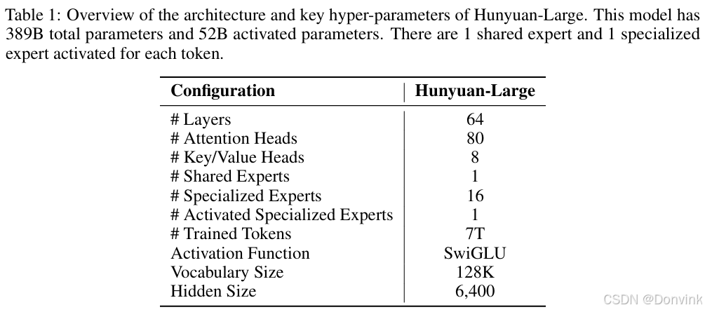
2.2.1 模型架构和超参

下表展示了Hunyuan-Large模型架构及其关键超参数：

2.2.2 KV缓存压缩

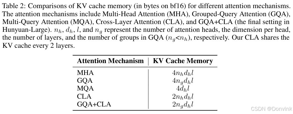
为了缓解KV缓存的内存压力并降低推理过程中的成本，Hunyuan-Large结合了两种经典的KV缓存压缩策略：

1. 分组查询注意力（Grouped-Query Attention, GQA）：这种方法使用中等数量的KV头形成 head groups，从头的角度压缩KV缓存。具体来说，GQA通过减少实际需要存储的KV头的数量来实现这一目标。在Hunyuan-Large中，我们设置了8组KV头用于GQA。

2. 跨层注意力（Cross-Layer Attention, CLA）：该方法在相邻层之间共享KV缓存，从而从层的角度进行压缩。这种方式可以减少每一层所需的KV缓存量，进一步节省内存。在Hunyuan-Large中，每两层之间共享KV缓存。

这两种技术共同作用，在保证有效性和效率的同时显著减少了内存使用。下表展示了不同机制下的KV缓存内存使用情况对比。在Hunyuan-Large中采用的GQA+CLA技术相比原始的多头注意力（MHA）机制总共节省了近95%的KV缓存，极大地提高了推理效率，同时对模型性能的影响很小。

2.2.3 专家路由策略

1. 共享专家与特殊专家（ Shared and Specialized Experts）

在MoE架构中，专家路由策略对于高效激活每个专家的能力同时保持相对平衡的负载至关重要。传统的路由策略，如经典的top-k路由策略，会选择得分最高的前k个专家来处理每个token。Hunyuan-Large采用了一种混合路由策略，结合了所有token共享的一个共享专家和几个使用经典top-k路由策略的可路由专家。

• 共享专家：Hunyuan-Large设置了一个共享专家，用于捕捉所有token所需的共同知识。
• 专门专家：此外，还分配了16个专门的专家来动态学习领域特定的知识，为每个token激活得分最高的一个特殊专家。

2. 回收路由

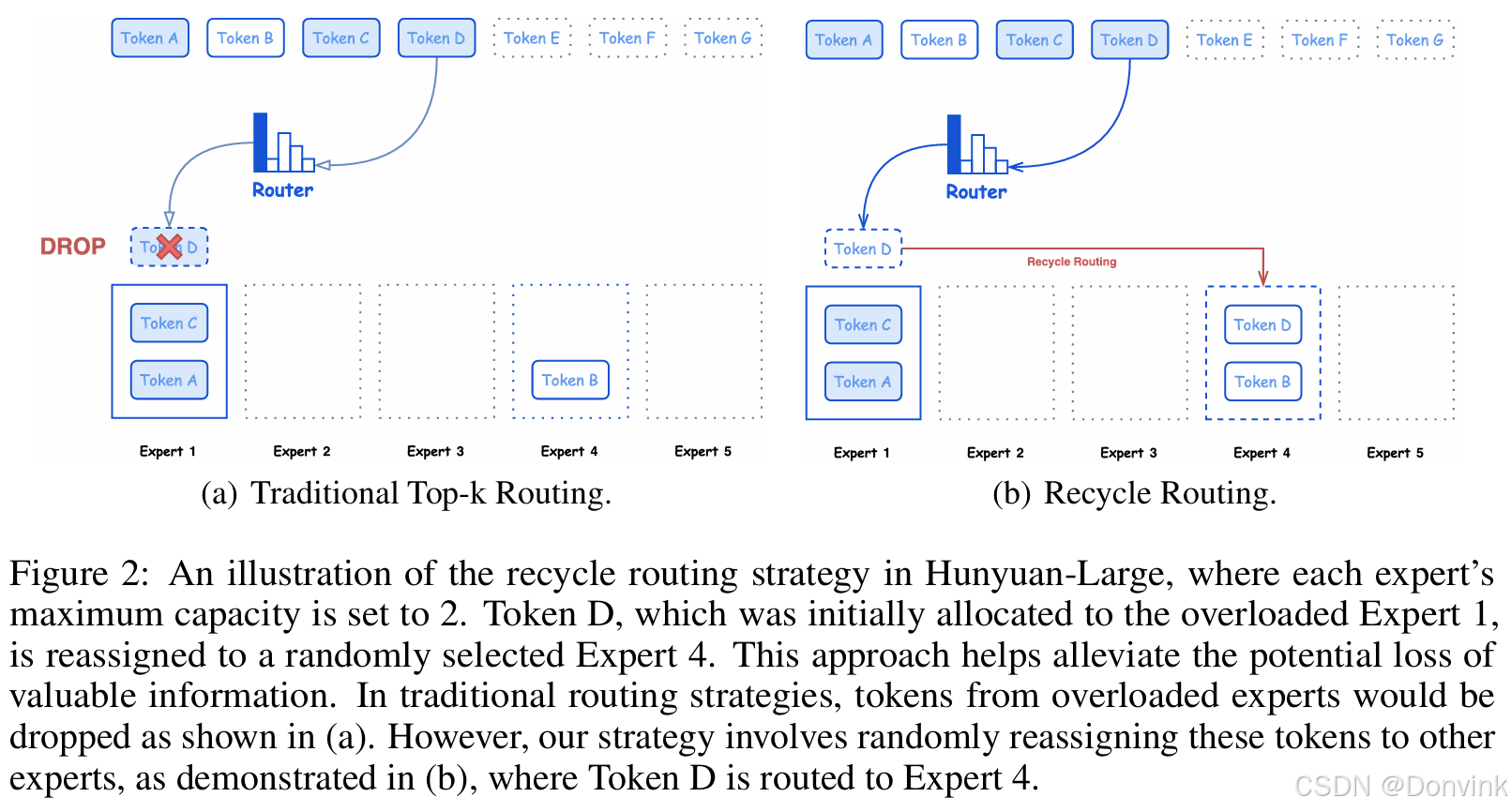
传统的top-k路由通常与容量因子配合使用，容量因子决定了MoE中每个专家的最大负载。在这种情况下，当专家过载时，其部分token会被丢弃。容量因子越大，丢弃的token越少，但会降低训练效率。过度丢弃token可能会导致关键信息的丢失，从而对训练稳定性产生负面影响。

为了解决这个问题，并在效率和稳定性之间实现更平衡的训练，作者开发了一种新的回收路由策略，用于处理在原始top-k路由过程中被丢弃的token，下图所示。该技术涉及对最初路由到过载专家的token进行额外的随机分配，将其重新分配给未超过容量的其他特殊专家。这种方法旨在保留重要信息的同时优化训练效率，从而确保模型训练的整体有效性和效率。

2.2.4 专家特定的学习率缩放

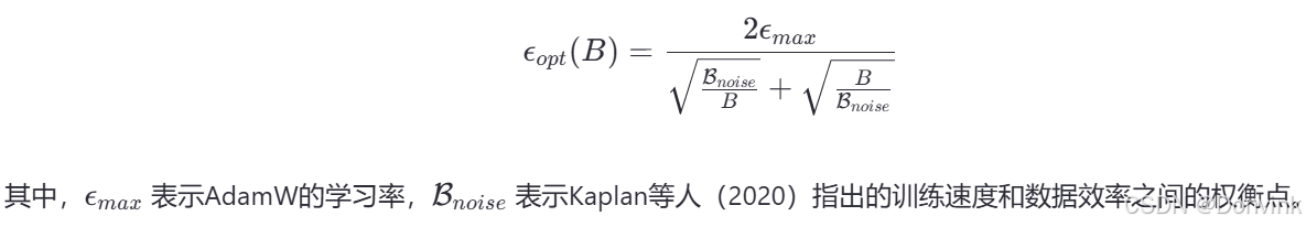
作者采用AdamW作为优化器，为了加快训练速度，在预训练过程中随着批量大小的增长相应地增加学习率。先前的研究在基于批量大小为SGD优化器寻找最优学习率时，探索了平方根缩放或线性缩放。最近的工作阐明了对于LLM中的Adam优化器，最优学习率和批量大小之间更合适的关系。根据Li等人（2024a），对于批量大小 B 的最优学习率 epsilon_opt(B) 的计算公式如下：

但是在Hunyuan-Large中，不同专家在训练token方面存在不平衡（例如，共享专家与其他专家相比）。每个专家在单次迭代中处理的token数量会有所不同，这意味着每个专家在一次训练迭代中会经历不同的有效批量大小。因此，有必要采用专家特定的学习率来优化训练效率。考虑到负载平衡损失，可以假设不同的特殊专家具有大致相同的有效训练token数量，因此，对于特殊专家，有效批量大小应除以特殊专家的数量，从而得出它们的最优学习率为 （Hunyuan激活16个特殊专家中的1个，因此 n = 16 ）。共享专家与特殊专家之间的学习率缩放比为 ，在Hunyuan中大约为0.31。因此，在配置Hunyuan-Large的学习率时，为共享专家分配最优学习率为 ，并有意降低专门专家的学习率。

2.3 预训练策略

LLM预训练的效果不仅取决于数据集和模型结构，还依赖于从经验实验中获得的预训练丹方。作者首先探讨MoE模型的扩展定律（Scaling Law），作为模型设计的指南。然后，介绍退火和长上下文预训练的详细过程，这些过程进一步增强了LLM的能力。

2.3.1 MoE扩展定律

通常，密集模型的训练计算预算（计算资源总量）可通过 C = 6ND 来估计，其中 N 表示参数数量，D 表示训练token数。然而，对于具有更长序列（如8K、32K和256K）的MoE模型，由于注意力复杂性和稀疏激活，计算预算的公式有所不同。经过仔细计算，作者确定了MoE模型的精确计算预算 C，其中公式中的 N 代表激活参数的数量：

C ≈ 9.59ND + 2.3 × 10⁸D

批量大小 B 对训练期间的计算预算 C 有显著影响，为了隔离这种效应并得出精确估计，作者使用了关键批量大小 B_crit(L)，它优化了时间与计算效率之间的权衡，最终最小计算预算 C_min为：

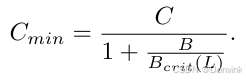
总的来说，这个公式是关于计算预算和批量大小之间关系，为Hunyuan-Large模型的设计和优化提供了重要的参考依据。通过这种分析，研究者可以更精确地确定在特定批量大小下模型的最优计算预算，以实现成本效益最大化。

作者做了一系列分析，这些分析确保了Hunyuan-Large在尽可能好的成本效益下达到最优性能，同时也促进了未来一系列MoE模型的发展。

2.3.2 学习率调度

一个好的学习率调度（Schedule）对于有效的稳定训练至关重要，Hunyuan-Large的学习率调度分为三个连续的阶段：初始升温阶段，随后是一个长时间的逐渐衰减阶段，并以一个简短的退火阶段结束。

通过在初始预训练阶段保持较高的学习率，模型可以有效地遍历解决方案空间的不同区域，从而避免过早收敛到次优局部最小值。随着训练进程逐步减少学习率确保系统地向更优解收敛。

在最后5%预训练token中，作者引入了一个简短的退火阶段，在此期间学习率被降低到其峰值的十分之一。这种方法有助于模型细致地微调其参数，从而实现更高程度的泛化，进而提升整体性能。此外，在这个阶段，作者会优先使用最高质量的数据集，这对于增强模型在退火阶段的表现起到了关键作用。

2.3.3 长上下文预训练

退火阶段之后，Hunyuan-Large会在更长的序列（最多256K标记）上进行训练，以增强其长上下文能力。具体来说，长上下文预训练阶段包含两个阶段（即逐渐增加标记长度至32K→256K）。作者使用旋转位置嵌入RoPE，并在256K预训练阶段将RoPE的基础频率扩展至10亿。

对于数据，仅依赖从书籍和代码中获得的自然长上下文数据（约占语料库的25%），并将其与正常长度的预训练数据（约75%）混合，形成长上下文预训练语料库。

作者发现，LLM获取长上下文能力并不需要太多的训练，在32K和256K每个阶段中，都使用大约100亿个token的长上下文预训练语料库。

2.4 后训练（Post-Training）

这一阶段包含监督微调（SFT）和从人类反馈中进行强化学习（RLHF）两个部分。

2.4.1 SFT

SFT的表现强依赖于与各种LLM能力相关的高质量指令数据。在SFT中，作者专注于详细的数据收集和处理方法以及SFT的训练设置，以确保Hunyuan-Large后训练的有效性。

整个SFT数据量超过100万。数据选择、预处理和训练过程主要步骤如下：

• 指令提取。作者开发了一个专门针对数学、逻辑推理和基于知识的问答等领域的指令抽取模型，其主要目标是从公开的可用数据源(如网页、百科全书等)中有效地提取适合于指令调整的数据。提取的数据包括指令和相应的参考答案。
• 指令泛化。作者设计并训练了一个指令概括系统，该系统能够在逐步增加目标指令的难度和复杂性的同时对其进行概括。这个系统的中心配方在于通过合成简单和复杂指令之间的大量映射来训练模型。此外，构建了一个结构良好的指令分类法及其相应的分类模型，旨在分析和平衡各种指令类型在SFT数据中的分布。
• 指令平衡。通过指令提取和泛化过程，作者积累了超过1000万条指令。然而，许多生成的指令具有非常相似的语义，指令类型分布自然是不平衡的。为了提高指令复杂度，同时保持均衡的指令分布，作者为每条指令附加标签。这些标签包含多个尺寸。通过仔细标记这些标签，作者可以更准确地理解和分析指令集的特性。通过在SFT过程中保证不同类型指令的数量充足和均衡分布，可以有效缓解特定指令类型的过拟合或欠拟合问题，从而提高模型的泛化能力和对不同应用场景的适应性
• 数据质量控制。作者主要通过以下三种方法来保证SFT数据的高质量。
  • 基于规则的过滤。作者发现了SFT数据中的一些常见问题，如数据截断错误、重复、乱码和格式错误。因此，作者开发了一套基于规则的数据过滤策略，以防止上述指令提取和生成模型产生不良输出。
  • 基于模型的过滤。为了从大量合成的指令数据中自动提取高质量的SFT数据，作者基于混元系列的70B稠密模型训练了一个批评性模型，该模型为每个指令样本分配一个四级质量分数，评估生成的答复的准确性、相关性、完整性、有用性和清晰度等方面，以及其他可能的数据质量问题。
  • 基于人工的过滤。在模型训练之前，通过基于规则和基于模型的方法过滤的SFT数据进一步经过人工注释，确保答案符合期望的任务特定响应模式，并避免引入额外的低质量问题。

在SFT中，作者根据高质量数据（超过100万）对预训练模型进行微调，共3个epoch。

2.4.2 RLHF

为了使Hunyuan-Large与人类偏好保持一致，作者使用DPO进一步训练SFT模型。

作者采用了一种结合离线和在线训练的单阶段训练策略，利用预先编译的偏好数据集来增强可控性，同时使用当前策略模型为每个提示生成多个响应，并通过奖励模型选择最受欢迎和最不受欢迎的响应。

为了增强训练稳定性，在选择的响应上引入了一个SFT损失项，这一措施有助于稳定的DPO训练，防止所选响应的log概率下降。此外，作者采用了指数移动平均策略以缓解reward hacking并减少 alignment tax，确保在一个更大规模的数据集上实现更稳定的训练过程。

3 关键源码分析（MoE）

混元大模型的代码其实和其他MoE模型差不多，结构比较清晰，适合上手。

3.1 HunYuanForCausalLM

model是Hunyuan模型，lm_head是将模型输出结果映射到词表长度的线性层，用于预测概率。

def __init__(self, config: HunYuanConfig):
    super().__init__(config)
    self.model = HunYuanModel(config)
    self.vocab_size = config.vocab_size
    self.lm_head = nn.Linear(config.hidden_size, config.vocab_size, bias=False)

forward()函数运行模型并预测每个词的概率，以及计算训练时的损失函数。

class HunYuanForCausalLM(HunYuanPreTrainedModel):
    
    def forward(...) -> Union[Tuple, CausalLMOutputWithPast]:
        
        # 1.配置信息
        output_attentions = output_attentions if output_attentions is not None else self.config.output_attentions
        output_hidden_states = (
            output_hidden_states if output_hidden_states is not None else self.config.output_hidden_states
        )
        return_dict = return_dict if return_dict is not None else self.config.use_return_dict
 
        # 2.模型输出 decoder outputs consists of (dec_features, layer_state, dec_hidden, dec_attn)
        outputs = self.model(       # HunYuanModel
            input_ids=input_ids,
            attention_mask=attention_mask,
            position_ids=position_ids,
            past_key_values=past_key_values,
            inputs_embeds=inputs_embeds,
            use_cache=use_cache,
            output_attentions=output_attentions,
            output_hidden_states=output_hidden_states,
            return_dict=return_dict,
        )
 
        # 3.线性层预测概率（分多卡和单卡版）
        hidden_states = outputs[0]
        if self.config.pretraining_tp > 1:  # 多卡并行
            # 按pretraining_tp分成多个部分
            lm_head_slices = self.lm_head.weight.split(self.vocab_size // self.config.pretraining_tp, dim=0)
            # 对每个部分进行线性变换，得到多个logits
            logits = [F.linear(hidden_states, lm_head_slices[i]) for i in range(self.config.pretraining_tp)]
            # 在最后一个维度上拼接起来
            logits = torch.cat(logits, dim=-1)
        else:  # 单卡
            logits = self.lm_head(hidden_states)
        logits = logits.float()
 
        # 4.计算Loss
        loss = None
        if labels is not None:      # 自回归损失函数计算
            # Shift so that tokens < n predict n  将 logits 的最后一个维度去掉一位，labels 则去掉第一个维度的第一位，使 logits 的每个位置预测下一个位置的 label
            shift_logits = logits[..., :-1, :].contiguous()
            shift_labels = labels[..., 1:].contiguous()
            # Flatten the tokens  展平 tokens
            loss_fct = CrossEntropyLoss()
            shift_logits = shift_logits.view(-1, self.config.vocab_size)
            shift_labels = shift_labels.view(-1)
            # Enable model parallelism
            shift_labels = shift_labels.to(shift_logits.device)
            # 计算损失
            loss = loss_fct(shift_logits, shift_labels)
 
        if not return_dict:
            output = (logits,) + outputs[1:]
            return (loss,) + output if loss is not None else output
 
        # 5.返回结果
        return CausalLMOutputWithPast(
            loss=loss,
            logits=logits,
            past_key_values=outputs.past_key_values,
            hidden_states=outputs.hidden_states,
            attentions=outputs.attentions,
        )

3.2 HunYuanModel

模型的核心层由许多HunYuanDecoderLayer组成，代码中还设置了attention的计算方法、归一化层的方法等。

class HunYuanModel(HunYuanPreTrainedModel):
    def __init__(self, config: HunYuanConfig):
        super().__init__(config)
        self.padding_idx = config.pad_token_id
        self.vocab_size = config.vocab_size
 
        self.embed_tokens = nn.Embedding(config.vocab_size, config.hidden_size, self.padding_idx)
        # 核心层
        self.layers = nn.ModuleList(
            [HunYuanDecoderLayer(config, layer_idx) for layer_idx in range(config.num_hidden_layers)]        
        )
        self._use_sdpa = config._attn_implementation == "sdpa"
        self._use_flash_attention_2 = config._attn_implementation == "flash_attention_2"
        self.norm = HunYuanRMSNorm(config.hidden_size, eps=config.rms_norm_eps)
 
        self.cla = config.use_cla
        self.cla_share_factor = config.cla_share_factor
 
        self.gradient_checkpointing = False
        # Initialize weights and apply final processing
        self.post_init()

其forward()函数如下，先生成注意力掩码和位置信息等信息，然后调用每一层的decoder_layer进行处理，并保存中间结果（如隐藏状态和注意力权重），最后输出结果。

class HunYuanModel(HunYuanPreTrainedModel):
    @add_start_docstrings_to_model_forward(HUNYUAN_INPUTS_DOCSTRING)
    def forward(...) -> Union[Tuple, BaseModelOutputWithPast]:
        # 此处省略初始化部分
 
        past_key_values_length = 0
        if use_cache:
            use_legacy_cache = not isinstance(past_key_values, Cache)
            # 是否使用kv-cache
            if use_legacy_cache:
                past_key_values = DynamicCache.from_legacy_cache(past_key_values)
            past_key_values_length = past_key_values.get_usable_length(seq_length)
 
        # 嵌入位置信息
        if position_ids is None:
            device = input_ids.device if input_ids is not None else inputs_embeds.device
            position_ids = torch.arange(
                past_key_values_length, seq_length + past_key_values_length, dtype=torch.long, device=device
            )
            position_ids = position_ids.unsqueeze(0)
 
        # embedding
        if inputs_embeds is None:
            inputs_embeds = self.embed_tokens(input_ids)
        
        # Fix lora with gradient checkpointing training
        if self.training and inputs_embeds.is_leaf:
            inputs_embeds.requires_grad = True
 
        if self._use_flash_attention_2:
            # 2d mask is passed through the layers，选择注意力掩码
            attention_mask = attention_mask if (attention_mask is not None and 0 in attention_mask) else None
        elif self._use_sdpa and not output_attentions:
            # output_attentions=True can not be supported when using SDPA, and we fall back on
            # the manual implementation that requires a 4D causal mask in all cases.
            attention_mask = _prepare_4d_causal_attention_mask_for_sdpa(
                attention_mask,
                (batch_size, seq_length),
                inputs_embeds,
                past_key_values_length,
            )
        else:
            # 4d mask is passed through the layers
            attention_mask = _prepare_4d_causal_attention_mask(
                attention_mask, (batch_size, seq_length), inputs_embeds, past_key_values_length
            )
 
        # embed positions
        hidden_states = inputs_embeds
 
        # decoder layers
        all_hidden_states = () if output_hidden_states else None
        all_self_attns = () if output_attentions else None
        next_decoder_cache = None
 
        prev_kv_states = None
        for layer_idx, decoder_layer in enumerate(self.layers):     # 多层解码器进行计算
            if output_hidden_states:
                all_hidden_states += (hidden_states,)
 
            if self.gradient_checkpointing and self.training:
                layer_outputs = self._gradient_checkpointing_func(
                    decoder_layer.__call__,
                    hidden_states,
                    attention_mask,
                    position_ids,
                    past_key_values,
                    output_attentions,
                    use_cache,
                    prev_kv_states,
                )
            else:
                layer_outputs = decoder_layer(
                    hidden_states,
                    attention_mask=attention_mask,
                    position_ids=position_ids,
                    past_key_value=past_key_values,
                    output_attentions=output_attentions,
                    use_cache=use_cache,
                    kv_states=prev_kv_states
                )
                
            # 保存中间结果，如隐藏状态和注意力权重。
            hidden_states = layer_outputs[0]
 
            if use_cache:       # KV-cache
                next_decoder_cache = layer_outputs[2 if output_attentions else 1]
 
            if output_attentions:       # 注意力权重。
                all_self_attns += (layer_outputs[1],)
 
            kv_states = layer_outputs[-1]       # kv
 
            if self.cla and layer_idx % self.cla_share_factor == 0:
                prev_kv_states = kv_states
 
        hidden_states = self.norm(hidden_states)
 
        # 输出，add hidden states from the last decoder layer
        if output_hidden_states:
            all_hidden_states += (hidden_states,)
 
        next_cache = None
        if use_cache:
            next_cache = next_decoder_cache.to_legacy_cache() if use_legacy_cache else next_decoder_cache
        if not return_dict:
            return tuple(v for v in [hidden_states, next_cache, all_hidden_states, all_self_attns] if v is not None)
        return BaseModelOutputWithPast(
            last_hidden_state=hidden_states,
            past_key_values=next_cache,
            hidden_states=all_hidden_states,
            attentions=all_self_attns,
        )

父类里面定义了初始化操作：

class HunYuanPreTrainedModel(PreTrainedModel):
    ...
 
    def _init_weights(self, module):
        std = self.config.initializer_range
        # 线性层使用正态分布初始化权重，并将偏置项设置为零
        if isinstance(module, nn.Linear): 
            module.weight.data.normal_(mean=0.0, std=std)
            if module.bias is not None:
                module.bias.data.zero_()
        # Embedding使用正态分布初始化权重，并将指定的填充索引位置的权重设置为零
        elif isinstance(module, nn.Embedding):
            module.weight.data.normal_(mean=0.0, std=std)
            if module.padding_idx is not None:
                module.weight.data[module.padding_idx].zero_()

3.3 DecoderLayer

混元模型的注意力有不同的模式，在同一文件下定义了三个类，可以自行选择，包括HunYuanAttention（原始注意力）、HunYuanFlashAttention2和HunYuanSdpaAttention。

MLP层根据num_experts的值选择HunYuanMoE或者HunYuanMLP；归一化使用的是HunYuanRMSNorm。

class HunYuanDecoderLayer(nn.Module):
    def __init__(self, config: HunYuanConfig, layer_idx: int):
        super().__init__()
        self.hidden_size = config.hidden_size
        self.layer_idx = layer_idx
 
        self.self_attn = HUNYUAN_ATTENTION_CLASSES[config._attn_implementation](config=config, layer_idx=layer_idx)
 
        if config.num_experts > 1:
            self.mlp = HunYuanMoE(config, layer_idx=layer_idx)
        else:
            self.mlp = HunYuanMLP(config, layer_idx=layer_idx, is_shared_mlp=False)
        self.input_layernorm = HunYuanRMSNorm(config.hidden_size, eps=config.rms_norm_eps)
        self.post_attention_layernorm = HunYuanRMSNorm(config.hidden_size, eps=config.rms_norm_eps)

forward方法和普通的decoder差不多。

class HunYuanDecoderLayer(nn.Module):
    def forward(...) -> Tuple[torch.FloatTensor, Optional[Tuple[torch.FloatTensor, torch.FloatTensor]]]:
        ...
 
        residual = hidden_states
 
        # 输入归一化
        hidden_states = self.input_layernorm(hidden_states)
 
        # Self Attention
        hidden_states, self_attn_weights, present_key_value, kv_states = self.self_attn(
            hidden_states=hidden_states,
            attention_mask=attention_mask,
            position_ids=position_ids,
            past_key_value=past_key_value,
            output_attentions=output_attentions,
            use_cache=use_cache,
            kv_states=kv_states,
            **kwargs,
        )
        # 残差连接
        hidden_states = residual + hidden_states
 
        # Fully Connected
        residual = hidden_states
        # 后注意力归一化
        hidden_states = self.post_attention_layernorm(hidden_states)
        # 全连接层
        hidden_states = self.mlp(hidden_states)
        # 残差连接
        hidden_states = residual + hidden_states
 
        outputs = (hidden_states,)
 
        # 是否输出注意力权重
        if output_attentions:
            outputs += (self_attn_weights,)
 
        # 是否输出缓存
        if use_cache: 
            outputs += (present_key_value,)
 
        # 返回键值状态
        outputs += (kv_states,)
 
        return outputs

3.4 RoPE

定义的原版RoPE类：

# RoPE旋转位置编码
class HunYuanRotaryEmbedding(nn.Module):
    def __init__(self, dim, max_position_embeddings=2048, base=10000, device=None):
        super().__init__()
 
        self.dim = dim
        self.max_position_embeddings = max_position_embeddings
        self.base = base
        inv_freq = 1.0 / (self.base ** (torch.arange(0, self.dim, 2).float().to(device) / self.dim))    # 计算逆频率 inv_freq
        inv_freq = inv_freq.bfloat16()
        # 注册缓冲区：使用 self.register_buffer 方法将计算结果注册为模型的缓冲区变量，并且设置 persistent=False 表示这个缓冲区不会被保存在模型的状态字典中。
        self.register_buffer("inv_freq", inv_freq, persistent=False)
 
        # Build here to make `torch.jit.trace` work.
        # 调用 _set_cos_sin_cache 方法预计算缓存
        self._set_cos_sin_cache(
            seq_len=max_position_embeddings, device=self.inv_freq.device, dtype=torch.get_default_dtype()
        )
 
    def _set_cos_sin_cache(self, seq_len, device, dtype):
        self.max_seq_len_cached = seq_len
        # 根据输入序列长度 seq_len，计算时间步长 t
        t = torch.arange(self.max_seq_len_cached, device=device, dtype=torch.float32)
 
        # 计算两个张量的外积freqs
        freqs = torch.outer(t, self.inv_freq)
        # Different from paper, but it uses a different permutation in order to obtain the same calculation
        # 拼接成 emb
        emb = torch.cat((freqs, freqs), dim=-1).float()
        # 计算并缓存 cos 和 sin 值
        self.register_buffer("cos_cached", emb.cos().to(dtype), persistent=False)
        self.register_buffer("sin_cached", emb.sin().to(dtype), persistent=False)
 
    def forward(self, x, seq_len=None):
        # x: [bs, num_attention_heads, seq_len, head_size]
        # 如果超过最大缓存长度，则更新缓存
        if seq_len > self.max_seq_len_cached:
            self._set_cos_sin_cache(seq_len=seq_len, device=x.device, dtype=x.dtype)
 
        return (
            self.cos_cached[:seq_len].to(dtype=x.dtype),
            self.sin_cached[:seq_len].to(dtype=x.dtype),
        )

核心代码如下：

# 应用RoPE
def apply_rotary_pos_emb(q, k, cos, sin, position_ids, unsqueeze_dim=1):
    cos = cos[position_ids].unsqueeze(unsqueeze_dim)
    sin = sin[position_ids].unsqueeze(unsqueeze_dim)
    q_embed = (q * cos) + (rotate_half(q) * sin)
    k_embed = (k * cos) + (rotate_half(k) * sin)
    return q_embed, k_embed

# 旋转
def rotate_half(x):
    """Rotates half the hidden dims of the input."""
    x1 = x[..., : x.shape[-1] // 2]
    x2 = x[..., x.shape[-1] // 2:]
    return torch.cat((-x2, x1), dim=-1)

3.5 repeat_kv

复制key和value张量，对应前文提到的KV缓存压缩。

输入：hidden_states是形状为 (batch, num_key_value_heads, seqlen, head_dim) 的四维张量。

输出：将张量的形状调整为 (batch, num_attention_heads, seqlen, head_dim)，其中 num_attention_heads = num_key_value_heads * n_rep。

# 在特定维度上重复张量
def repeat_kv(hidden_states: torch.Tensor, n_rep: int) -> torch.Tensor:
    """
    This is the equivalent of torch.repeat_interleave(x, dim=1, repeats=n_rep). The hidden states go from (batch,
    num_key_value_heads, seqlen, head_dim) to (batch, num_attention_heads, seqlen, head_dim)
    """
    batch, num_key_value_heads, slen, head_dim = hidden_states.shape
    if n_rep == 1:
        return hidden_states
    # 使用 expand 方法在新的维度上扩展张量，使其形状变为 (batch, num_key_value_heads, n_rep, seqlen, head_dim)
    hidden_states = hidden_states[:, :, None, :, :].expand(batch, num_key_value_heads, n_rep, slen, head_dim)
    # 将张量的形状调整为 (batch, num_attention_heads, seqlen, head_dim)，其中 num_attention_heads = num_key_value_heads * n_rep
    return hidden_states.reshape(batch, num_key_value_heads * n_rep, slen, head_dim)

3.6 HunYuanMOE

3.6.1 HunYuanMLP

这个MLP层是由门控层和两层线性层组成，其运算过程：out = down(act(gate(x))*up(x))，其中，x是输入，out是输出，up和down分别为两层线性层，gate为门控层，act为激活函数。

class HunYuanMLP(nn.Module):
    def __init__(self, config: HunYuanConfig, layer_idx=None, is_shared_mlp=False):
        super().__init__()
        self.config = config
        self.layer_idx = layer_idx
        self.hidden_size = config.hidden_size
        if is_shared_mlp:
            self.intermediate_size = config.intermediate_size * config.num_shared_expert
        else:
            self.intermediate_size = config.intermediate_size
        # 门控层
        self.gate_proj = nn.Linear(self.hidden_size, self.intermediate_size, bias=False)
        self.up_proj = nn.Linear(self.hidden_size, self.intermediate_size, bias=False)
        self.down_proj = nn.Linear(self.intermediate_size, self.hidden_size, bias=False)
        self.act_fn = ACT2FN[config.hidden_act]
 
    def forward(self, x):
        if self.config.pretraining_tp > 1:      # 多卡
            # 权重矩阵按照指定的切片大小进行分割
            slice = self.intermediate_size // self.config.pretraining_tp
            gate_proj_slices = self.gate_proj.weight.split(slice, dim=0)
            up_proj_slices = self.up_proj.weight.split(slice, dim=0)
            down_proj_slices = self.down_proj.weight.split(slice, dim=1)
 
            # 对输入 x 进行多次线性变换，并将结果在最后一个维度上拼接起来
            gate_proj = torch.cat(
                [F.linear(x, gate_proj_slices[i]) for i in range(self.config.pretraining_tp)], dim=-1
            )
            up_proj = torch.cat([F.linear(x, up_proj_slices[i]) for i in range(self.config.pretraining_tp)], dim=-1)
 
            intermediate_states = (self.act_fn(gate_proj) * up_proj).split(slice, dim=2)
            down_proj = [
                F.linear(intermediate_states[i], down_proj_slices[i]) for i in range(self.config.pretraining_tp)
            ]
            down_proj = sum(down_proj)
        else:       # 单卡
            down_proj = self.down_proj(self.act_fn(self.gate_proj(x)) * self.up_proj(x))
 
        return down_proj

3.6.2 HunYuanMoE

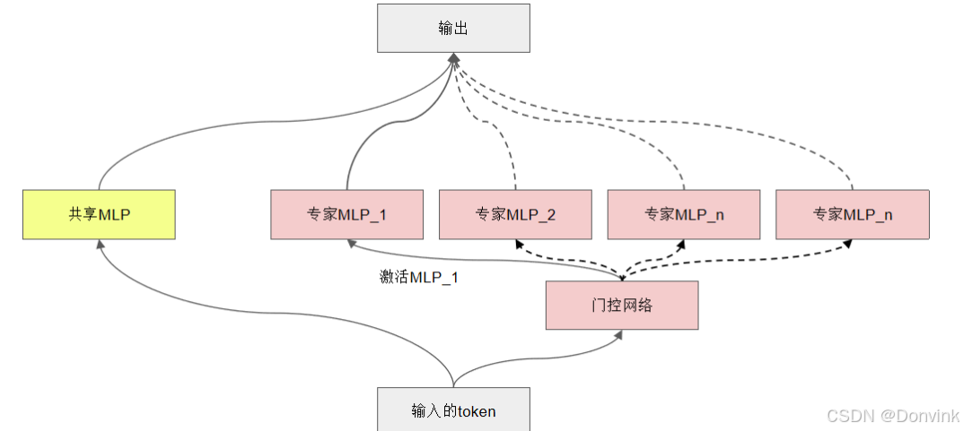
MoE具体步骤：

• 如果有共享的MLP层，输入数据先经过共享MLP，得到hidden_states_mlp
• 通过门控层(HunYuanTopKGate)计算每个专家的负载
• 拆分输入数据，然后将不同数据交给不同的专家进行处理，得到expert_outputs
  • 根据dispatch_mask，使用torch.einsum分配给不同的专家
  • 使用沿第一个维度（通常是批次维度）切分成self.num_experts个块，每个块对应一个专家的处理输入
  • 遍历每个块和专家，计算输出
• 将不同专家的输出拼起来，并恢复原来的形状，得到combined_output
• 如果有共享的MLP层，将专家输出结果和共享MLP的输出拼起来
• 返回结果

class HunYuanMoE(nn.Module):
    def __init__(self, config: HunYuanConfig, layer_idx: Optional[int] = None):
        super().__init__()
        self.config = config
        self.layer_idx = layer_idx
        self.moe_topk = config.moe_topk
        self.num_experts = config.num_experts
        # 创建共享 MLP 层
        if config.use_mixed_mlp_moe:
            self.shared_mlp = HunYuanMLP(config, layer_idx=layer_idx, is_shared_mlp=True)
        # 门控机制
        self.gate = HunYuanTopKGate(config, layer_idx=layer_idx)
        # 创建专家
        self.experts = nn.ModuleList(
            [HunYuanMLP(config, layer_idx=layer_idx, is_shared_mlp=False) for _ in range(config.num_experts)]
        )
 
    def forward(self, hidden_states):
        bsz, seq_len, hidden_size = hidden_states.shape
 
        # 对输入进行共享MLP处理
        if self.config.use_mixed_mlp_moe:
            hidden_states_mlp = self.shared_mlp(hidden_states)
 
        # 门控计算每个专家的分配权重和掩码
        l_moe, combine_weights, dispatch_mask, exp_counts = self.gate(hidden_states)
 
        reshaped_input = hidden_states.reshape(-1, hidden_size)
 
        # 根据掩码将输入分派给不同的专家
        # [s,num_expect,容量],[s,hidden_size]->[num_expect,容量,hidden_size]
        dispatched_input = torch.einsum("sec,sm->ecm", dispatch_mask.type_as(hidden_states), reshaped_input)
        # 按专家数量切分，每个专家处理一个输入部分
        chunks = dispatched_input.chunk(self.num_experts, dim=0)
        expert_outputs = []
 
 		# 每个专家处理分派给它的输入部分
        for chunk, expert in zip(chunks, self.experts):
            expert_outputs.append(expert(chunk))
 
        # 将专家的输出重新组合成原始输入的形状
        expert_output = torch.cat(expert_outputs, dim=0)
        # [s,num_expect,容量],[num_expect,容量,hidden_size]->[s,hidden_size]
        combined_output = torch.einsum("sec,ecm->sm", combine_weights.type_as(hidden_states), expert_output)
        combined_output = combined_output.reshape(bsz, seq_len, hidden_size)
 
        if self.config.use_mixed_mlp_moe:
            # 混合MLP输出与组合输出相加
            output = hidden_states_mlp + combined_output
        else: 
        	# 如果没有启用混合MLP模式，直接返回组合后的专家输出
            output = combined_output
 
        return output

3.6.3 HunYuanTopKGate

门控机制负责决定每个输入token应该被分配给哪些专家进行处理，即根据模型配置和输入的隐藏状态，计算每个token分配给不同专家的概率，并据此进行路由。

class HunYuanTopKGate(nn.Module):
    def __init__(self, config: HunYuanConfig, layer_idx: Optional[int] = None):
        super().__init__()
        self.config = config
        self.layer_idx = layer_idx
        self.moe_topk = config.moe_topk
        self.drop_tokens = config.moe_drop_tokens
        self.min_capacity = 8
        self.random_routing_dropped_token = config.moe_random_routing_dropped_token
        # 用于将hidden_size映射到专家数量
        self.wg = nn.Linear(config.hidden_size, config.num_experts, bias=False, dtype=torch.float32)
 
    def forward(self, hidden_states):
        bsz, seq_len, hidden_size = hidden_states.shape
        hidden_states = hidden_states.reshape(-1, hidden_size)
        if self.wg.weight.dtype == torch.float32:
            hidden_states = hidden_states.float()
        # 通过线性层 self.wg 计算门控逻辑 logits
        logits = self.wg(hidden_states)
        if self.moe_topk == 1:
            gate_output = top1gating(logits, random_routing_dropped_token=self.random_routing_dropped_token)
        else:
            # Top-K路由机制
            gate_output = topkgating(logits, self.moe_topk)
 
        return gate_output

3.6.4 路由机制 topkgating()

这个函数是整个路由机制的核心，允许每个token被分配给概率最高的前k个专家，提供了一种更加灵活的路由策略，可以在模型的负载均衡和处理能力之间取得平衡。

返回值：

• dispatch_mask 是一个布尔掩码，用于指示每个token应该被发送到哪些专家。
• combine_weights 是用于合并专家输出的权重

dispatch_mask 计算步骤：

• 首先，计算每个token的优先级，这个优先级是基于token被分配到专家的顺序。
• 通过使用one-hot编码，将每个token的专家索引转换为一个掩码，指示该token是否被分配给特定的专家。
• 接下来，生成一个有效掩码，确保每个token的优先级在有效范围内（即优先级非负且小于专家的容量）。
• 然后，将这个有效掩码应用到优先级上，填充无效的优先级值为0。最后，将优先级转换为one-hot编码形式，生成最终的dispatch_mask，这个掩码的形状通常为 (tokens_per_group, num_experts, expert_capacity)，指示每个token在每个专家的缓存中应该占据的位置。

这个过程确保了每个token只被路由到其优先级有效且不超过专家容量的专家，从而实现了高效的负载分配和输出合并。

combine_weights 的计算过程：

• 首先，通过softmax函数将logits（即每个token分配给每个专家的原始分数）转换成概率分布，这些概率表示每个token被分配到每个专家的可能性。

• 接着，计算每个token分配给所有专家的总概率（gates_s），这个总概率是通过对softmax概率进行求和得到的。

• 然后，对softmax概率进行归一化处理，得到每个token分配给每个专家的归一化概率（router_probs）。这是通过将softmax概率除以每个token分配给所有专家的总概率来实现的，目的是确保每个token分配给所有专家的归一化概率之和为1。

• 接下来，使用torch.topk函数从归一化概率中选择每个token的前topk个最可能的专家，并将这些选择转换为one-hot编码形式的掩码（dispatch_mask），这个掩码指示每个token应该被发送到哪些专家。

• 最后，通过torch.einsum函数结合归一化的门控信号（router_probs）和调度掩码（dispatch_mask）来计算combine_weights。这个操作实际上是将每个token的归一化概率与它应该被发送到的每个专家的调度掩码相乘，得到一个四维数组，其中包含了每个token对于每个专家输出的贡献权重。

combine_weights 的形状通常是 (num_groups, tokens_per_group, num_experts, expert_capacity)，其中 num_groups 是批次中的组数，tokens_per_group 是每个组中的token数，num_experts 是专家的数量，expert_capacity 是每个专家的容量。这个权重数组在后续步骤中用于将各个专家的输出按照它们对每个token的贡献权重合并起来，形成最终的模型输出。这样，每个专家只对其被分配的token贡献输出，而没有被分配的token则不包含在该专家的输出中。

def topkgating(logits: Tensor, topk: int):
    logits = logits.float()     # 线性层hidden_size -> num_expects的结果，[s,m=num_expects]
    gates = F.softmax(logits, dim=1)    # 计算每个token对每个专家的路由概率。
    expert_capacity = topk * gates.shape[0]
    num_experts = int(gates.shape[1])
    # Top-k router probability and corresponding expert indices for each token.
    # Shape: [tokens_per_group, num_selected_experts].
    expert_gate, expert_index = torch.topk(gates, topk)     # 使用 torch.topk 确定每个token的Top-K专家及其对应的路由概率。
    expert_mask = F.one_hot(expert_index, num_experts)      # 使用 F.one_hot 生成专家掩码
    # For a given token, determine if it was routed to a given expert.
    # Shape: [tokens_per_group, num_experts]
    expert_mask_aux = expert_mask.max(dim=-2)[0]
    tokens_per_group_and_expert = torch.mean(expert_mask_aux.float(), dim=-2)   # 计算每个专家的负载
    router_prob_per_group_and_expert = torch.mean(gates.float(), dim=-2)
    l_aux = num_experts**2 * torch.mean(tokens_per_group_and_expert * router_prob_per_group_and_expert)     # 生成辅助损失 l_aux
 
    # 计算每个token的优先级
    gates_s = torch.clamp(      # 计算专家门控权重的加权和，并对其进行裁剪，确保结果不会小于一个极小值。
        torch.matmul(expert_mask.float(), gates.unsqueeze(-1)).sum(dim=1), min=torch.finfo(gates.dtype).eps
    )
    router_probs = gates / gates_s      # 计算路由概率
    # Make num_selected_experts the leading axis to ensure that top-1 choices have priority over top-2 choices, which have priority over top-3 choices, etc.
    expert_index = torch.transpose(expert_index, 0, 1)
    expert_index = expert_index.reshape(-1)     # Shape: [num_selected_experts * tokens_per_group]
 
    # Create mask out of indices.
    expert_mask = F.one_hot(expert_index, num_experts).to(torch.int32)     # 计算每个专家被选择的次数 Shape: [tokens_per_group * num_selected_experts, num_experts].
    exp_counts = torch.sum(expert_mask, dim=0).detach()     # 计算每个专家被选择的次数
 
    # 计算每个令牌在目标专家中的优先级。Experts have a fixed capacity that we cannot exceed. A token's priority within the expert's buffer is given by the masked, cumulative capacity of its target expert.
    # Shape: [tokens_per_group * num_selected_experts, num_experts].
    token_priority = torch.cumsum(expert_mask, dim=0) * expert_mask - 1
    # Shape: [num_selected_experts, tokens_per_group, num_experts].
    token_priority = token_priority.reshape((topk, -1, num_experts))
    # Shape: [tokens_per_group, num_selected_experts, num_experts].
    token_priority = torch.transpose(token_priority, 0, 1)
    # For each token, across all selected experts, select the only non-negative (unmasked) priority. Now, for group G routing to expert E, token T has non-negative priority (i.e. token_priority[G,T,E] >= 0) if and only if E is its targeted expert.
    # Shape: [tokens_per_group, num_experts].
    token_priority = torch.max(token_priority, dim=1)[0]        # 在所有选择的专家中，选择唯一的非负优先级。
 
    # 生成有效的调度掩码
    # Token T can only be routed to expert E if its priority is positive and less than the expert capacity. One-hot matrix will ignore indices outside the range [0, expert_capacity).
    # Shape: [tokens_per_group, num_experts, expert_capacity].
    valid_mask = torch.logical_and(token_priority >= 0, token_priority < expert_capacity)   # 布尔张量 valid_mask，标记了token_priority中在[0, expert_capacity)范围内的元素。
    token_priority = torch.masked_fill(token_priority, ~valid_mask, 0)      # 将 token_priority 中不在有效范围内的值设为 0。
    dispatch_mask = F.one_hot(token_priority, expert_capacity).to(torch.bool)   # 将 token_priority 转换为 one-hot 编码，生成 dispatch_mask
    valid_mask = valid_mask.unsqueeze(-1).expand(-1, -1, expert_capacity)
    dispatch_mask = torch.masked_fill(dispatch_mask, ~valid_mask, 0)    # 将 dispatch_mask 中对应 valid_mask 为 False 的位置设为 0。
 
    # The combine array will be used for combining expert outputs, scaled by the router probabilities. Shape: [num_groups, tokens_per_group, num_experts, expert_capacity].
    combine_weights = torch.einsum("...te,...tec->...tec", router_probs, dispatch_mask)
    exp_counts_capacity = torch.sum(dispatch_mask)      # 计算调度掩码的期望容量
    exp_capacity_rate = exp_counts_capacity / (logits.shape[0]*topk)    # 计算容量利用率
    return [l_aux, exp_capacity_rate], combine_weights, dispatch_mask, exp_counts

3.6.5 top1gating()

top1gating 函数的目的是实现基于 logits 的 Top-1 门控机制，选择每个 token 最优的专家（expert），并计算辅助损失 l_aux 和专家容量利用率 exp_capacity_rate。该函数还处理随机路由丢弃的 token，确保每个专家的负载均衡。

• 识别未满专家：首先，通过计算每个专家的容量与已分配token的数量差，找出那些尚未达到容量上限的专家。

• 重新分配被丢弃token：然后，将那些未被分配给任何专家的token随机分配给上述未满的专家，以此来优化专家的负载均衡，并确保所有token都能得到处理。

def top1gating(logits: Tensor, random_routing_dropped_token: bool = False):
    """Implements Top1Gating on logits."""
    # everything is in fp32 in this function
    logits = logits.float()
    gates = F.softmax(logits, dim=1)    # 计算门控概率
    capacity = gates.shape[0]
 
    # Create a mask for 1st's expert per token
    # noisy gating
    indices1_s = torch.argmax(gates, dim=1)     # 选择最佳专家
    num_experts = int(gates.shape[1])
    mask1 = F.one_hot(indices1_s, num_classes=num_experts)
 
    # gating decisions
    # exp_counts = torch.sum(mask1, dim=0).detach().to('cpu')
    exp_counts = torch.sum(mask1, dim=0).detach()
 
    # Compute l_aux     计算辅助损失
    me = torch.mean(gates, dim=0)
    ce = torch.mean(mask1.float(), dim=0)
    l_aux = torch.sum(me * ce) * num_experts
    mask1_rand = mask1
 
    top_idx = torch.topk(mask1_rand, k=capacity, dim=0)[1]
 
    new_mask1 = mask1 * torch.zeros_like(mask1).scatter_(0, top_idx, 1)
    mask1 = new_mask1
    mask1_bk = mask1
    if random_routing_dropped_token:        # 随机路由丢弃  处理丢弃的token，重新分配给未满的专家
        not_full = capacity - new_mask1.sum(dim=0)   # 计算每个专家剩余的容量
        sorted_notfull, indices_notfull = torch.sort(not_full, descending=True)    # 对未满的专家进行排序
        sorted_notfull = sorted_notfull.to(torch.int64)
        not_full_experts_ids = torch.repeat_interleave(indices_notfull, sorted_notfull)    # 重复未满专家的索引
        shuffle_not_full_ids = torch.randperm(not_full_experts_ids.shape[0])    # 随机打乱未满专家的索引
        # 重新分配被丢弃的token
        not_full_experts_ids = not_full_experts_ids[shuffle_not_full_ids]    #  计算 new_mask1 中每个token被分配到的专家索引
        indices1_s_after_drop = torch.argmax(new_mask1, dim=1)
        # get drop idx
        drop_mask = 1 - new_mask1.sum(dim=1)    # 标识出那些没有被分配给任何专家的token（即被丢弃的token）
        drop_mask = drop_mask.bool()
        drop_idx = drop_mask.nonzero().view(-1)    # 获取被丢弃token的索引
        drop_num = drop_mask.sum().to(torch.int64)    # 计算被丢弃token的数量
        indices1_s_after_drop.scatter_(0, drop_idx, not_full_experts_ids[:drop_num])    # 将随机选择的未满专家索引分配给被丢弃的token
        nodrop_mask1 = F.one_hot(indices1_s_after_drop, num_classes=num_experts)    #  将更新后的专家索引转换为one-hot编码形式。
        mask1 = nodrop_mask1    # 每个token都被分配给了至少一个专家。
 
    # Compute locations in capacity buffer      计算位置索引
    locations1 = torch.cumsum(mask1, dim=0) - 1
 
    # Store the capacity location for each token
    locations1_s = torch.sum(locations1 * mask1, dim=1)
 
    # Normalize gate probabilities  归一化门控概率
    mask1_float = mask1.float()
    gates = gates * mask1_float
 
    # 归一化门控概率
    locations1_sc = F.one_hot(locations1_s, num_classes=capacity).float()   # one hot to float
    combine_weights = torch.einsum("se,sc->sec", gates, locations1_sc)
 
    dispatch_mask = combine_weights.bool()
 
    exp_counts_capacity = torch.sum(mask1_bk)
    exp_capacity_rate = exp_counts_capacity / (logits.shape[0])
    return [l_aux, exp_capacity_rate], combine_weights, dispatch_mask, exp_counts